caffe项目

https://zhuanlan.zhihu.com/p/24343706

https://chenrudan.github.io/blog/2015/05/07/cafferead.html

https://blog.csdn.net/jinzhuojun/article/details/79834697

https://blog.csdn.net/seven_first/article/details/47378697

https://blog.csdn.net/idevede/article/details/78606832

https://blog.csdn.net/lanxuecc/article/details/53219666

https://www.zhihu.com/question/27982282

https://blog.csdn.net/langb2014/article/details/50988275?locationNum=5&fps=1

一、protobuf教程

1.1 protocol buffers是什么

Protocol buffers是一种语言中立,平台无关,可扩展的序列化数据的格式,可用于通信协议,数据存储等。

Protocol buffers在序列化数据方面,它是灵活的,高效的。相比于XML来说,Protocol buffers更加小巧,更加快速,更加简单。一旦定义了要处理的数据的数据结构之后,就可以利用Protocol buffers的代码生成工具生成相关的代码。甚至可以在无需重新部署程序的情况下更新数据结构。只需使用Protobuf对数据结构进行一次描述,即可利用各种不同语言或从各种不同数据流中对你的结构化数据轻松读写。

Protocol buffers很适合做数据存储或RPC数据交换格式。可用于通讯协议、数据存储等领域的语言无关、平台无关、可扩展的序列化结构数据格式。

为什么要发明protocol buffers?

大家可能会觉得Google发明protocol buffers是为了解决序列化速度的,其实真实的原因并不是这样的。protocol buffers最先开始是google用来解决索引服务器request/response协议的。没有protocol buffers之前,google已经存在了一种request/response格式,用于手动处理request/response的编组和反编组。它也能支持多版本协议,不过代码比较丑陋:

if (version == 3) {
    ...
} else if (version > 4) {
    if (version == 5) {
        ...
    }
    ...
}

如果非常明确的格式化协议,会使新协议变得非常复杂。因为开发人员必须确保请求发起者与处理请求的实际服务器之间的所有服务器都能理解新协议,然后才能切换开关以开始使用新协议。这也就是每个服务器开发人员都遇到过的低版本兼容、新旧协议兼容相关的问题。protocol buffers为了解决这些问题,于是就诞生了。protocol buffers被寄予一下2个特点:

可以很容易地引入新的字段,并且不需要检查数据的中间服务器可以简单地解析并传递数据,而无需了解所有字段。

数据格式更加具有自我描述性,可以用各种语言来处理(C++,Java等各种语言)

这个版本的protocol buffers仍需要自己手写解析的代码。

不过随着系统慢慢发展,演进,protocol buffers目前具有了更多的特性:

自动生成的序列化和反序列化代码避免了手动解析的需要。(官方提供自动生成代码工具,各个语言平台的基本都有)

除了用于RPC(远程过程调用)请求之外,人们开始将protocol buffers用作持久存储数据的便捷自描述格式(例如,在Bigtable中)。

服务器的RPC接口可以先声明为协议的一部分,然后用protocol compiler生成基类,用户可以使用服务器接口的实际实现来覆盖它们。

protocol buffers现在是Google用于数据的通用语言。在撰写本文时,谷歌代码树中定义了48162种不同的消息类型,包括12183个 .proto文件。它们既用于RPC系统,也用于在各种存储系统中持久存储数据。

1.2 proto3定义message

proto2和proto3的名字看起来有点扑朔迷离,那是因为当我们最初开源的protocol buffers时,它实际上是Google的第二个版本了,所以被称为proto2,这也是我们的开源版本号从v2开始的原因。初始版名为proto1,从2001年初开始在谷歌开发的。在proto中,所有结构化的数据都被称为message。

message helloworld {
    required int32     id = 1;  // ID
    required string    str = 2;  // str
    optional int32     opt = 3;  //optional field
}

上面这几行语句,定义了一个消息helloworld,该消息有三个成员,类型为int32的 id,另一个为类型为string的成员str。opt是一个可选的成员,即消息中可以不包含该成员。接下来说明一些proto3中需要注意的地方。

syntax = "proto3";

message SearchRequest {
    string query = 1;
    int32 page_number = 2;
    int32 result_per_page = 3;
}

如果开头第一行不声明syntax="proto3";,则默认使用proto2进行解析。

required:字段必须提供,否则消息将被认为是"未初始化的(uninitialized)"。如果libprotobuf以debug模式编译,则序列化未初始化的消息将导致断言失败。在优化的构建中,检查将被跳过,消息仍将被写入。然而,解析未初始化的消息将总是失败(通过喜爱parse方法中返回false)。否则,required字段的行为将与optional字段完全相同。

optional:字段可以设置也可以不设置。如果可选的字段值没有设置,则将使用默认值。对于简单的类型,你可以指定你自己的默认值,如我们在例子中为电话号码类型做的那样。否则,将使用系统默认值:数字类型为0,字符串类型为空字符串,bools值为false。对于内嵌的消息,默认值总是消息的"默认实例(defaultinstance)"或 "原型(prototype)",它们没有自己的字段集。调用accessor获取还没有显式地设置的optional (或required)字段的值总是返回字段的默认值。

repeated:字段可以重复任意多次(包括0)。在protocol buffer中,重复值的顺序将被保留。将重复字段想象为动态大小的数组。

分配字段编号

每个消息定义中的每个字段都有唯一的编号。这些字段编号用于标识消息二进制格式中的字段,并且在使用消息类型后不应更改。请注意,范围1到15中的字段编号需要一个字节进行编码,包括字段编号和字段类型。范围16至2047中的字段编号需要两个字节。所以你应该保留数字1到15作为非常频繁出现的消息元素。请记住为将来可能添加的频繁出现的元素留出一些空间。

可以指定的最小字段编号为1,最大字段编号为 $2^{29}-1$ 或536,870,911。也不能使用数字19000到19999(FieldDescriptor::kFirstReservedNumber到FieldDescriptor::kLastReservedNumber),因为它们是为Protocol Buffers实现保留的。如果在.proto中使用这些保留数字中的一个,Protocol Buffers编译的时候会报错。同样,您不能使用任何以前Protocol Buffers保留的一些字段号码。

保留字段

如果您通过完全删除某个字段或将其注释掉来更新消息类型,那么未来的用户可以在对该类型进行自己的更新时重新使用该字段号。如果稍后加载到了的旧版本.proto文件,则会导致服务器出现严重问题,例如数据混乱,隐私错误等等。确保这种情况不会发生的一种方法是指定删除字段的字段编号(或名称,这也可能会导致JSON序列化问题)为reserved。如果将来的任何用户试图使用这些字段标识符,Protocol Buffers编译器将会报错。

message Foo {
    reserved 2, 15, 9 to 11;
    reserved "foo", "bar";
}

注意,不能在同一个reserved语句中混合字段名称和字段编号。如有需要需要像上面这个例子这样写。

默认字段规则

字段名不能重复,必须唯一。repeated字段:可以在一个message中重复任何数字多次(包括0),不过这些重复值的顺序被保留。在proto3中,纯数字类型的repeated字段编码时候默认采用packed编码。

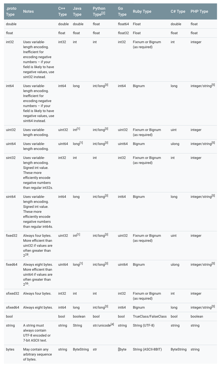
各个语言标量类型对应关系

枚举

在message中可以嵌入枚举类型。

message SearchRequest {
    string query = 1;
    int32 page_number = 2;
    int32 result_per_page = 3;
    enum Corpus {
            UNIVERSAL = 0;
            WEB = 1;
            IMAGES = 2;
            LOCAL = 3;
            NEWS = 4;
            PRODUCTS = 5;
            VIDEO = 6;
    }
    Corpus corpus = 4;
}

枚举类型需要注意的是,一定要有0值。枚举为0的是作为零值,当不赋值的时候,就会是零值。为了和proto2兼容。在proto2中,零值必须是第一个值。

另外在反序列化的过程中,无法被识别的枚举值,将会被保留在messaage中。因为消息反序列化时如何表示是依赖于语言的。在支持指定符号范围之外的值的开放枚举类型的语言中,例如C++和 Go,未知的枚举值只是存储为其基础整数表示。在诸如Java之类的封闭枚举类型的语言中,枚举值会被用来标识未识别的值,并且特殊的访问器可以访问到底层整数。在其他情况下,如果消息被序列化,则无法识别的值仍将与消息一起序列化。

枚举中的保留值

如果您通过完全删除枚举条目或将其注释掉来更新枚举类型,未来的用户可以在对该类型进行自己的更新时重新使用数值。如果稍后加载到了的旧版本.proto文件,则会导致服务器出现严重问题,例如数据混乱,隐私错误等等。确保这种情况不会发生的一种方法是指定已删除条目的数字值(或名称,这也可能会导致JSON序列化问题)为reserved。如果将来的任何用户试图使用这些字段标识符,Protocol Buffers编译器将会报错。您可以使用max关键字指定您的保留数值范围上升到最大可能值。

enum Foo {
    reserved 2, 15, 9 to 11, 40 to max;
    reserved "FOO", "BAR";
}

注意,不能在同一个reserved语句中混合字段名称和字段编号。如有需要需要像上面这个例子这样写。

允许嵌套

Protocol Buffers定义message允许嵌套组合成更加复杂的消息。

message SearchResponse {
    repeated Result results = 1;
}

message Result {
    string url = 1;
    string title = 2;
    repeated string snippets = 3;
}

上面的例子中,SearchResponse中嵌套使用了Result。更多的例子:

message SearchResponse {
    message Result {
            string url = 1;
            string title = 2;
            repeated string snippets = 3;
    }
    repeated Result results = 1;
  }

message SomeOtherMessage {
    SearchResponse.Result result = 1;
}
message Outer {                  // Level 0
    message MiddleAA {  // Level 1
            message Inner {   // Level 2
                int64 ival = 1;
                bool  booly = 2;
            }
    }
    message MiddleBB {  // Level 1
            message Inner {   // Level 2
                int32 ival = 1;
                bool  booly = 2;
            }
    }
}

枚举不兼容性

可以导入proto2消息类型并在proto3消息中使用它们,反之亦然。然而,proto2枚举不能直接用在proto3语法中(但是如果导入的proto2消息使用它们,这是可以的)。

更新message

如果后面发现之前定义message需要增加字段了,这个时候就体现出Protocol Buffer的优势了,不需要改动之前的代码。不过需要满足以下10条规则:

不要改动原有字段的数据结构。

如果您添加新字段,则任何由代码使用“旧”消息格式序列化的消息仍然可以通过新生成的代码进行分析。您应该记住这些元素的默认值,以便新代码可以正确地与旧代码生成的消息进行交互。同样,由新代码创建的消息可以由旧代码解析:旧的二进制文件在解析时会简单地忽略新字段。(具体原因见未知字段这一章节)

只要字段号在更新的消息类型中不再使用,字段可以被删除。您可能需要重命名该字段,可能会添加前缀“OBSOLETE_”,或者标记成保留字段号reserved,以便将来的.proto用户不会意外重复使用该号码。

int32,uint32,int64,uint64和 bool 全都兼容。这意味着您可以将字段从这些类型之一更改为另一个字段而不破坏向前或向后兼容性。如果一个数字从不适合相应类型的线路中解析出来,则会得到与在C++中将该数字转换为该类型相同的效果(例如,如果将64位数字读为int32,它将被截断为32位)。

sint32和sint64相互兼容,但与其他整数类型不兼容。

只要字节是有效的UTF-8,string和bytes是兼容的。

嵌入式message与 bytes兼容,如果bytes包含message的encodedversion。

fixed32与sfixed32兼容,而fixed64与sfixed64兼容。

enum就数组而言,是可以与int32,uint32,int64和uint64兼容(请注意,如果它们不适合,值将被截断)。但是请注意,当消息反序列化时,客户端代码可能会以不同的方式对待它们:例如,未识别的proto3枚举类型将保留在消息中,但消息反序列化时如何表示是与语言相关的。(这点和语言相关,上面提到过了)Int域始终只保留它们的值。

将单个值更改为新的成员是安全和二进制兼容的。如果您确定一次没有代码设置多个字段,则将多个字段移至新的字段可能是安全的。将任何字段移到现有字段中都是不安全的。(注意字段和值的区别,字段是field,值是value)

未知字段

未知数字段是protocol buffers序列化的数据,表示解析器无法识别的字段。例如,当一个旧的二进制文件解析由新的二进制文件发送的新数据的数据时,这些新的字段将成为旧的二进制文件中的未知字段。

Proto3实现可以成功解析未知字段的消息,但是,实现可能会或可能不会支持保留这些未知字段。你不应该依赖保存或删除未知域。对于大多数Googleprotocol buffers实现,未知字段在proto3中无法通过相应的proto运行时访问,并且在反序列化时被丢弃和遗忘。这是与proto2的不同行为,其中未知字段总是与消息一起保存并序列化。

Map类型

repeated类型可以用来表示数组,Map类型则可以用来表示字典。

map<key_type, value_type> map_field = N;
map<string, Project> projects = 3;

key_type可以是任何int或者string类型(任何的标量类型,具体可以见上面标量类型对应表格,但是要除去float、double和 bytes),枚举值也不能作为key。key_type可以是除去map以外的任何类型。

需要特别注意的是:

map是不能用repeated修饰的。

线性数组和map迭代顺序的是不确定的,所以你不能依靠你的map是在一个特定的顺序。

为.proto生成文本格式时,map按 key排序。数字的key按数字排序。

从数组中解析或合并时,如果有重复的key,则使用所看到的最后一个key(覆盖原则)。从文本格式解析映射时,如果有重复的key,解析可能会失败。

Protocol Buffer虽然不支持map类型的数组,但是可以转换一下,用以下思路实现maps数组:

message MapFieldEntry {
    key_type key = 1;
    value_type value = 2;
}
repeated MapFieldEntry map_field = N;

上述写法和map数组是完全等价的,所以用repeated巧妙的实现了maps数组的需求。

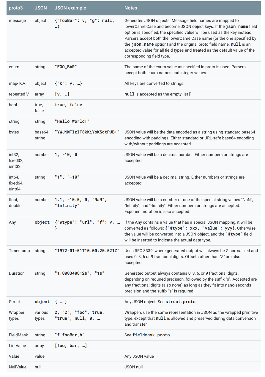
JSON Mapping

Proto3支持JSON中的规范编码,使系统之间共享数据变得更加容易。编码在下表中按类型逐个描述。

如果JSON编码数据中缺少值或其值为空,则在解析为protocol buffer时,它将被解释为适当的默认值。如果一个字段在协议缓冲区中具有默认值,默认情况下它将在JSON编码数据中省略以节省空间。具体Mapping的实现可以提供选项决定是否在JSON编码的输出中发送具有默认值的字段。

proto3的JSON实现中提供了以下4中options:

使用默认值发送字段:在默认情况下,默认值的字段在proto3 JSON输出中被忽略。一个实现可以提供一个选项来覆盖这个行为,并使用它们的默认值输出字段。

忽略未知字段:默认情况下,Proto3 JSON解析器应拒绝未知字段,但可能提供一个选项来忽略解析中的未知字段。

使用proto字段名称而不是lowerCamelCase名称:默认情况下,proto3 JSON的printer将字段名称转换为lowerCamelCase并将其用作JSON名称。实现可能会提供一个选项,将原始字段名称用作JSON名称。Proto3 JSON解析器需要接受转换后的lowerCamelCase名称和原始字段名称。

发送枚举形式的枚举值而不是字符串:在JSON输出中默认使用枚举值的名称。可以提供一个选项来使用枚举值的数值。

proto3定义Services

如果要使用RPC(远程过程调用)系统的消息类型,可以在.proto文件中定义RPC服务接口,protocol buffer编译器将使用所选语言生成服务接口代码和stubs。所以,例如,如果你定义一个RPC服务,入参是SearchRequest返回值是SearchResponse,你可以在你的.proto文件中定义它,如下所示:

service SearchService {
    rpc Search (SearchRequest) returns (SearchResponse);
}

与protocol buffer一起使用的最直接的RPC系统是gRPC:在谷歌开发的语言和平台中立的开源RPC系统。gRPC在protocol buffer中工作得非常好,并且允许你通过使用特殊的protocol buffer编译插件,直接从.proto文件中生成RPC相关的代码。

如果你不想使用gRPC,也可以在你自己的RPC实现中使用protocol buffers。您可以在Proto2语言指南中找到更多关于这些相关的信息。

还有一些正在进行的第三方项目为Protocol Buffers开发RPC实现。

Protocol Buffer命名规范

message采用驼峰命名法。message首字母大写开头。字段名采用下划线分隔法命名。

message SongServerRequest {
    required string song_name = 1;
}

枚举类型采用驼峰命名法。枚举类型首字母大写开头。每个枚举值全部大写,并且采用下划线分隔法命名。

enum Foo {
    FIRST_VALUE = 0;
    SECOND_VALUE = 1;
}

每个枚举值用分号结束,不是逗号。服务名和方法名都采用驼峰命名法。并且首字母都大写开头。

service FooService {
    rpc GetSomething(FooRequest) returns (FooResponse);
}

1.3 Protocol Buffer编码原理

在讨论Protocol Buffer编码原理之前,必须先谈谈Varints编码。

Base 128 Varints编码

Varint是一种紧凑的表示数字的方法。它用一个或多个字节来表示一个数字,值越小的数字使用越少的字节数。这能减少用来表示数字的字节数。

Varint中的每个字节(最后一个字节除外)都设置了最高有效位(msb),这一位表示还会有更多字节出现。每个字节的低7位用于以7位组的形式存储数字的二进制补码表示,最低有效组首位。

如果用不到1个字节,那么最高有效位设为0,如下面这个例子,1用一个字节就可以表示,所以msb为0.

0000 0001

如果需要多个字节表示,msb就应该设置为1。例如300,如果用Varint表示的话:

1010 1100 0000 0010

如果按照正常的二进制计算的话,这个表示的是88068(65536+16384+4096+2048+4)。

那Varint是怎么编码的呢?下面代码是Varint int32的编码计算方法。

char* EncodeVarint32(char* dst, uint32_t v) {
  // Operate on characters as unsigneds
  unsigned char* ptr = reinterpret_cast<unsigned char*>(dst);
  static const int B = 128;
  if (v < (1<<7)) {
    *(ptr++) = v;
  } else if (v < (1<<14)) {
    *(ptr++) = v | B;
    *(ptr++) = v>>7;
  } else if (v < (1<<21)) {
    *(ptr++) = v | B;
    *(ptr++) = (v>>7) | B;
    *(ptr++) = v>>14;
  } else if (v < (1<<28)) {
    *(ptr++) = v | B;
    *(ptr++) = (v>>7) | B;
    *(ptr++) = (v>>14) | B;
    *(ptr++) = v>>21;
  } else {
    *(ptr++) = v | B;
    *(ptr++) = (v>>7) | B;
    *(ptr++) = (v>>14) | B;
    *(ptr++) = (v>>21) | B;
    *(ptr++) = v>>28;
  }
  return reinterpret_cast<char*>(ptr);
}
// 300 = 100101100

由于300超过了7位(Varint一个字节只有7位能用来表示数字,最高位msb用来表示后面是否有更多字节),所以300需要用2个字节来表示。

Varint的编码,以300举例:

if (v < (1<<14)) {
    *(ptr++) = v | B;
    *(ptr++) = v>>7;
}

1. 100101100 | 10000000 = 1 1010 1100
2. 110101100 取出末尾 7 位 = 010 1100
3. 100101100 >> 7 = 10 = 0000 0010
4. 1010 1100 0000 0010 (最终 Varint 结果)

Varint的解码算法应该是这样的:(实际就是编码的逆过程)

如果是多个字节,先去掉每个字节的msb(通过逻辑或运算),每个字节只留下7 位。

逆序整个结果,最多是5 个字节,排序是1-2-3-4-5,逆序之后就是5-4-3-2-1,字节内部的二进制位的顺序不变,变的是字节的相对位置。

解码过程调用GetVarint32Ptr函数,如果是大于一个字节的情况,会调用GetVarint32PtrFallback来处理。

inline const char* GetVarint32Ptr(const char* p,
                                  const char* limit,
                                  uint32_t* value) {
  if (p < limit) {
    uint32_t result = *(reinterpret_cast<const unsigned char*>(p));
    if ((result & 128) == 0) {
      *value = result;
      return p + 1;
    }
  }
  return GetVarint32PtrFallback(p, limit, value);
}

const char* GetVarint32PtrFallback(const char* p,
                                   const char* limit,
                                   uint32_t* value) {
  uint32_t result = 0;
  for (uint32_t shift = 0; shift <= 28 && p < limit; shift += 7) {
    uint32_t byte = *(reinterpret_cast<const unsigned char*>(p));
    p++;
    if (byte & 128) {
      // More bytes are present
      result |= ((byte & 127) << shift);
    } else {
      result |= (byte << shift);
      *value = result;
      return reinterpret_cast<const char*>(p);
    }
  }
  return NULL;
}

至此,Varint处理过程读者应该都熟悉了。上面列举出了Varint32的算法,64位的同理,只不过不再用10个分支来写代码了,太丑了。(32位是5个字节,64位是10个字节)

64位Varint编码实现:

char* EncodeVarint64(char* dst, uint64_t v) {
  static const int B = 128;
  unsigned char* ptr = reinterpret_cast<unsigned char*>(dst);
  while (v >= B) {
    *(ptr++) = (v & (B-1)) | B;
    v >>= 7;
  }
  *(ptr++) = static_cast<unsigned char>(v);
  return reinterpret_cast<char*>(ptr);
}

原理不变,只不过用循环来解决了。

64位Varint解码实现:

const char* GetVarint64Ptr(const char* p, const char* limit, uint64_t* value) {
  uint64_t result = 0;
  for (uint32_t shift = 0; shift <= 63 && p < limit; shift += 7) {
    uint64_t byte = *(reinterpret_cast<const unsigned char*>(p));
    p++;
    if (byte & 128) {
      // More bytes are present
      result |= ((byte & 127) << shift);
    } else {
      result |= (byte << shift);
      *value = result;
      return reinterpret_cast<const char*>(p);
    }
  }
  return NULL;
}

读到这里可能有读者会问了,Varint不是为了紧凑int的么?那300本来可以用2个字节表示,现在还是2个字节了,哪里紧凑了,花费的空间没有变啊?！

Varint确实是一种紧凑的表示数字的方法。它用一个或多个字节来表示一个数字,值越小的数字使用越少的字节数。这能减少用来表示数字的字节数。比如对于int32类型的数字,一般需要4个 byte来表示。但是采用Varint,对于很小的int32类型的数字,则可以用1个 byte来表示。当然凡事都有好的也有不好的一面,采用Varint表示法,大的数字则需要5个 byte来表示。从统计的角度来说,一般不会所有的消息中的数字都是大数,因此大多数情况下,采用Varint后,可以用更少的字节数来表示数字信息。

300如果用int32表示,需要4 个字节,现在用Varint表示,只需要2 个字节了。缩小了一半！

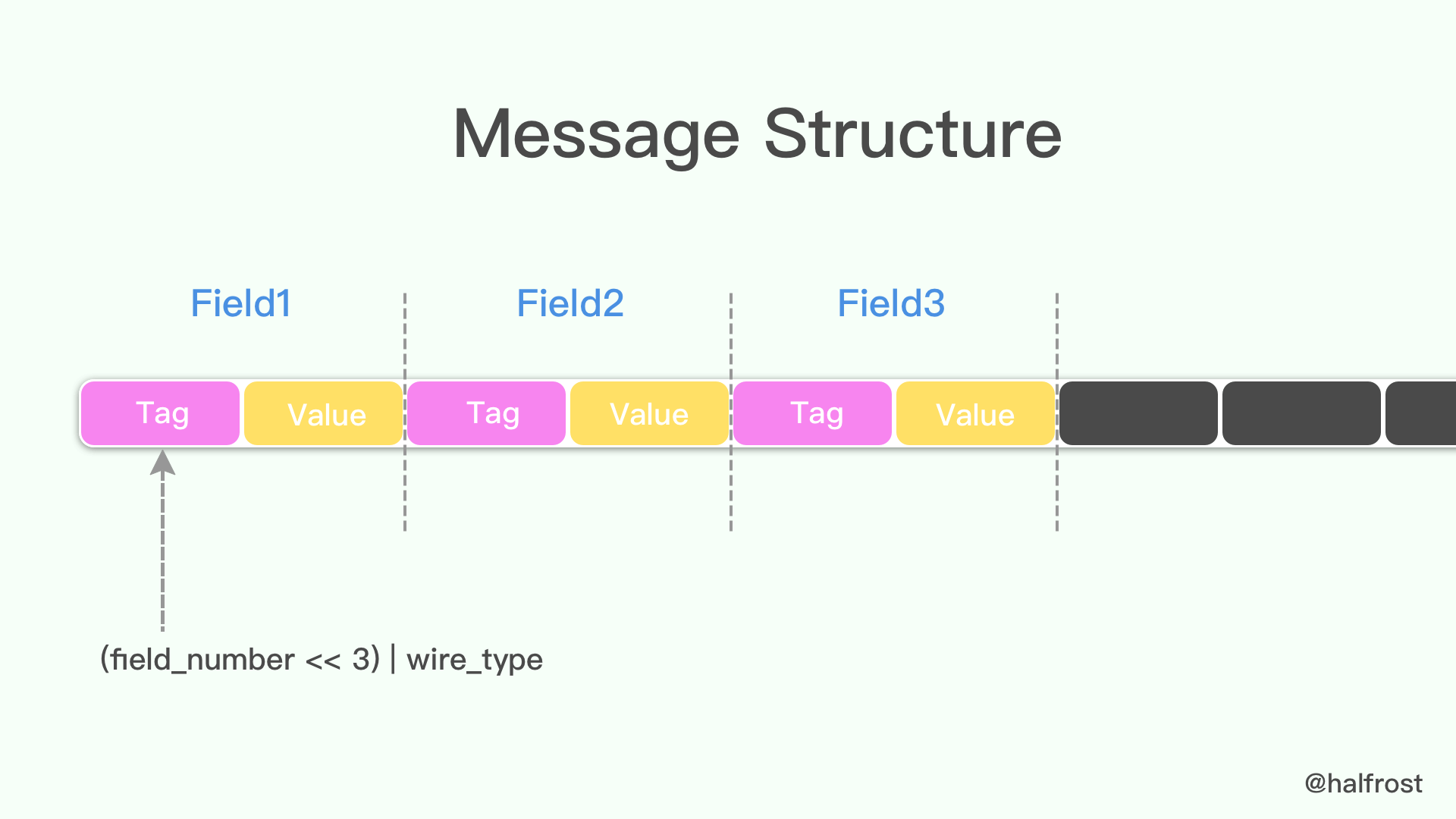
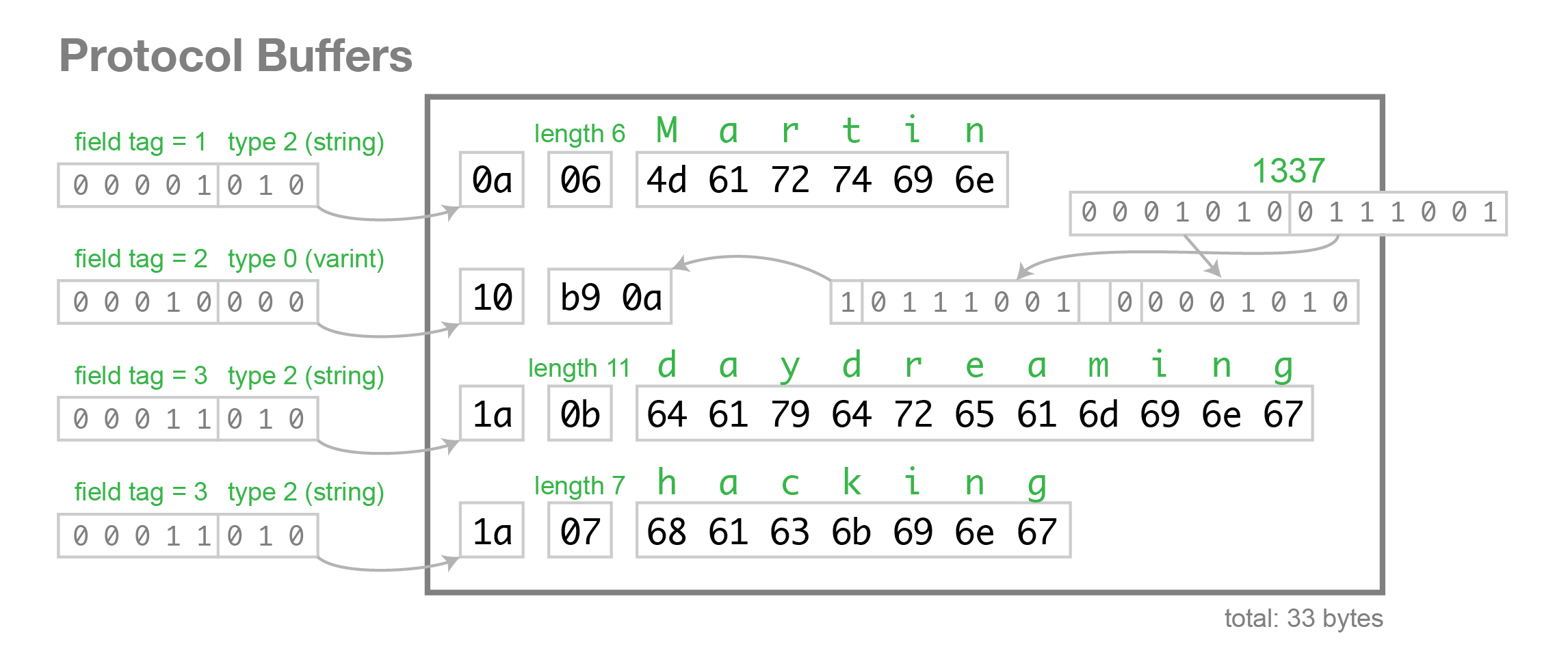
Message Structure编码

protocol buffer中message是一系列键值对。message的二进制版本只是使用字段号(field'snumber和wire_type)作为key。每个字段的名称和声明类型只能在解码端通过引用消息类型的定义(即.proto文件)来确定。这一点也是人们常常说的protocol buffer比JSON,XML安全一点的原因,如果没有数据结构描述.proto文件,拿到数据以后是无法解释成正常的数据的。

由于采用了tag-value的形式,所以option的 field如果有,就存在在这个message buffer中,如果没有,就不会在这里,这一点也算是压缩了message的大小了。

当消息编码时,键和值被连接成一个字节流。当消息被解码时,解析器需要能够跳过它无法识别的字段。这样,可以将新字段添加到消息中,而不会破坏不知道它们的旧程序。这就是所谓的“向后”兼容性。

为此,线性的格式消息中每对的“key”实际上是两个值,其中一个是来自.proto文件的字段编号,加上提供正好足够的信息来查找下一个值的长度。在大多数语言实现中,这个key被称为tag。

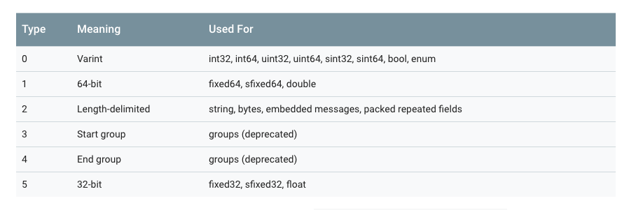
注意上图中,3和4已经被废弃了,所以wire_type取值目前只有0、1、2、5。

key的计算方法是(field_number<<3)|wire_type,换句话说,key的最后3位表示的就是wire_type。

举例,一般message的字段号都是1 开始的,所以对应的tag可能是这样的:

000 1000

末尾3 位表示的是value的类型,这里是000,即0 ,代表的是varint值。右移3 位,即0001,这代表的就是字段号(fieldnumber)。tag的例子就举这么多,接下来举一个value的例子,还是用varint来举例:

96 01 = 1001 0110  0000 0001
       → 000 0001  ++  001 0110 (drop the msb and reverse the groups of 7 bits)
       → 10010110
       → 128 + 16 + 4 + 2 = 150

可以96 01代表的数据就是150 。

message Test1 {
    required int32 a = 1;
}

如果存在上面这样的一个message的结构,如果存入150,在Protocol Buffer中显示的二进制应该为08 96 01。

额外说一句,type需要注意的是type= 2的情况,tag里面除了包含fieldnumber和 wire_type,还需要再包含一个length,决定value从那一段取出来。

Signed Integers编码

从上面的表格里面可以看到wire_type= 0中包含了无符号的varints,但是如果是一个无符号数呢?

一个负数一般会被表示为一个很大的整数,因为计算机定义负数的符号位为数字的最高位。如果采用Varint表示一个负数,那么一定需要10个byte长度。

为何32位和64位的负数都需要10个byte长度呢?

inline void CodedOutputStream::WriteVarint32SignExtended(int32 value) {
    WriteVarint64(static_cast<uint64>(value));
}

因为源码里面是这么规定的。32位的有符号数都会转换成64位无符号来处理。至于源码为什么要这么规定呢,猜想可能是怕32位的负数转换会有溢出的可能。(只是猜想)

为此GoogleProtocol Buffer定义了sint32这种类型,采用zigzag编码。将所有整数映射成无符号整数,然后再采用varint编码方式编码,这样,绝对值小的整数,编码后也会有一个较小的varint编码值。

Zigzag映射函数为:

Zigzag(n) = (n << 1) ^ (n >> 31), n 为 sint32 时
Zigzag(n) = (n << 1) ^ (n >> 63), n 为 sint64 时

按照这种方法,-1将会被编码成1,1将会被编码成2,-2会被编码成3,如下表所示:

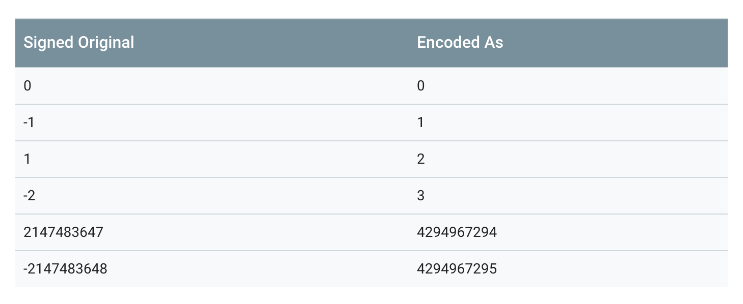
需要注意的是,第二个转换(n>>31)部分,是一个算术转换。所以,换句话说,移位的结果要么是一个全为0(如果n是正数),要么是全部1(如果n是负数)。

当sint32或 sint64被解析时,它的值被解码回原始的带符号的版本。

Non-varint Numbers

Non-varint数字比较简单,double、fixed64的wire_type为1,在解析时告诉解析器,该类型的数据需要一个64位大小的数据块即可。同理,float和fixed32的wire_type为5,给其32位数据块即可。两种情况下,都是高位在后,低位在前。

说Protocol Buffer压缩数据没有到极限,原因就在这里,因为并没有压缩float、double这些浮点类型。

字符串

wire_type类型为2 的数据,是一种指定长度的编码方式:key+length+content,key的编码方式是统一的,length采用varints编码方式,content就是由length指定长度的Bytes。

举例,假设定义如下的message格式:

message Test2 {
    optional string b = 2;
}

设置该值为"testing",二进制格式查看:

12 07 74 65 73 74 69 6e 67

74 65 73 74 69 6e 67 是“testing”的 UTF8 代码。

此处,key是16进制表示的,所以展开是:

12->0001 0010,后三位010为wire_type= 2,0001 0010右移三位为0000 0010,即tag = 2。

length此处为7,后边跟着7 个bytes,即我们的字符串"testing"。

所以wire_type类型为2 的数据,编码的时候会默认转换为T-L-V(Tag- Length- Value)的形式。

嵌入式message

假设,定义如下嵌套消息:

message Test3 {
    optional Test1 c = 3;
}

设置字段为整数150,编码后的字节为:

1a 03 08 96 01

08 96 01 这三个代表的是 150,上面讲解过,这里就不再赘述了。

1a->0001 1010,后三位010为wire_type = 2,0001 1010右移三位为0000 0011,即tag=3。

length为3,代表后面有3个字节,即08 96 01。

需要转变为T-L-V形式的还有string, bytes,embedded messages,packed repeated fields(即wire_type为2的形式都会转变成T-L-V形式)

Optional和Repeated的编码

在proto2中定义成repeated的字段,(没有加上[packed=true]option),编码后的message有一个或者多个包含相同tag数字的key-value对。这些重复的value不需要连续的出现;他们可能与其他的字段间隔的出现。尽管他们是无序的,但是在解析时,他们是需要有序的。在proto3中repeated字段默认采用packed编码。

对于proto3中的任何非重复字段或proto2中的可选字段,编码的message可能有也可能没有包含该字段号的键值对。

通常,编码后的message,其required字段和optional 字段最多只有一个实例。但是解析器却需要处理多对一的情况。对于数字类型和string类型,如果同一值出现多次,解析器接受最后一个它收到的值。对于内嵌字段,解析器合并(merge)它接收到的同一字段的多个实例。就如MergeFrom方法一样,所有单数的字段,后来的会替换先前的,所有单数的内嵌message都会被合并(merge),所有的repeated字段,都会串联起来。这样的规则的结果是,解析两个串联的编码后的message,与分别解析两个message然后merge,结果是一样的。例如:

MyMessage message;
message.ParseFromString(str1 + str2);

等价于

MyMessage message, message2;
message.ParseFromString(str1);
message2.ParseFromString(str2);
message.MergeFrom(message2);

这种方法有时是非常有用的。比如,即使不知道message的类型,也能够将其合并。

Packed Repeated Fields

在2.1.0版本以后,protocol buffers引入了该种类型,其与repeated字段一样,只是在末尾声明了[packed=true]。类似repeated字段却又不同。在proto3中 Repeated字段默认就是以这种方式处理。对于packedrepeated字段,如果message中没有赋值,则不会出现在编码后的数据中。否则的话,该字段所有的元素会被打包到单一一个key-value对中,且它的wire_type=2,长度确定。每个元素正常编码,只不过其前没有标签tag。例如有如下message类型:

message Test4 {
    repeated int32 d = 4 [packed=true];
}

构造一个Test4字段,并且设置repeated字段d 3个值:3,270和86942,编码后:

22 // tag 0010 0010(field number 010 0 = 4, wire type 010 = 2)
06 // payload size (设置的length = 6 bytes)
03 // first element (varint 3)
8E 02 // second element (varint 270)
9E A7 05 // third element (varint 86942)

形成了Tag- Length- Value- Value- Value……对。

只有原始数字类型(使用varint,32位或64位)的重复字段才可以声明为“packed”。

有一点需要注意,对于packed的 repeated字段,尽管通常没有理由将其编码为多个key-value对,编码器必须有接收多个key-pair对的准备。这种情况下,payload必须是串联的,每个pair必须包含完整的元素。

Protocol Buffer解析器必须能够解析被重新编译为packed的字段,就像它们未被packed一样,反之亦然。这允许以正向和反向兼容的方式将[packed= true]添加到现有字段。

Field Order

编码/解码与字段顺序无关,这一点由key-value机制保证。

如果消息具有未知字段,则当前的Java和C++实现在按顺序排序的已知字段之后以任意顺序写入它们。当前的Python实现不会跟踪未知字段。

1.3 protocol buffers的优缺点

protocol buffers 在序列化方面,与 XML 相比,有诸多优点:

更加简单

数据体积小 3- 10 倍

更快的反序列化速度,提高 20 - 100 倍

可以自动化生成更易于编码方式使用的数据访问类

举个例子:

如果要编码一个用户的名字和email信息,用XML的方式如下:

  <person>
    <name>John Doe</name>
    <email>jdoe@example.com</email>
  </person>

相同需求,如果换成protocol buffers来实现,定义文件如下:

# Textual representation of a protocol buffer.
# This is *not* the binary format used on the wire.
person {
  name: "John Doe"
  email: "jdoe@example.com"
}

protocol buffers通过编码以后,以二进制的方式进行数据传输,最多只需要28 bytes空间和100-200ns的反序列化时间。但是XML则至少需要69 bytes空间(经过压缩以后,去掉所有空格)和5000-10000的反序列化时间。

上面说的是性能方面的优势。接下来说说编码方面的优势。

protocol buffers自带代码生成工具,可以生成友好的数据访问存储接口。从而开发人员使用它来编码更加方便。例如上面的例子,如果用C++的方式去读取用户的名字和email,直接调用对应的get方法即可(所有属性的get和 set方法的代码都自动生成好了,只需要调用即可)

  cout << "Name: " << person.name() << endl;
  cout << "E-mail: " << person.email() << endl;

而XML读取数据会麻烦一些:

  cout << "Name: "
       << person.getElementsByTagName("name")->item(0)->innerText()
       << endl;
  cout << "E-mail: "
       << person.getElementsByTagName("email")->item(0)->innerText()
       << endl;

Protobuf语义更清晰,无需类似XML解析器的东西(因为Protobuf编译器会将.proto文件编译生成对应的数据访问类以对Protobuf数据进行序列化、反序列化操作)。

使用Protobuf无需学习复杂的文档对象模型,Protobuf的编程模式比较友好,简单易学,同时它拥有良好的文档和示例,对于喜欢简单事物的人们而言,Protobuf比其他的技术更加有吸引力。

protocol buffers最后一个非常棒的特性是,即“向后”兼容性好,人们不必破坏已部署的、依靠“老”数据格式的程序就可以对数据结构进行升级。这样您的程序就可以不必担心因为消息结构的改变而造成的大规模的代码重构或者迁移的问题。因为添加新的消息中的field并不会引起已经发布的程序的任何改变(因为存储方式本来就是无序的,k-v形式)。

当然protocol buffers也并不是完美的,在使用上存在一些局限性。

由于文本并不适合用来描述数据结构,所以Protobuf也不适合用来对基于文本的标记文档(如HTML)建模。另外,由于XML具有某种程度上的自解释性,它可以被人直接读取编辑,在这一点上Protobuf不行,它以二进制的方式存储,除非你有.proto定义,否则你没法直接读出Protobuf的任何内容。

1.4 Python使用Protobuf

用一个例子说明使用Python操作PB的方法:

定义.proto文件。

编译.proto文件产出Python代码。

使用Python API读写message。

该例子完成一个地址簿程序,能够对地址簿信息进行读写,地址簿中每个人的信息包括姓名、ID、email、联系电话。

// 定义addressbook.proto:
syntax = "proto3";
package tutorial;

message Person {
    string name = 1;
    int32 id = 2;
    string email = 3;

    enum PhoneType {
        MOBILE = 0;
        HOME = 1;
        WORK = 2;
    }

    message PhoneNumber {
        string number = 1;
        PhoneType type = 2;
    }
    repeated PhoneNumber phones = 4;
}

message AddressBook {
    repeated Person people = 1;
}

编译Protocol buffer: protoc --python_out=. addressbook.proto和生成addressbook_pb2.py

使用Python的Protobuf API

在Python脚本中使用addressbook_pb2.py:

import addressbook_pb2 as addressbook

person = addressbook.Person()
person.id = 1234
person.name = "John Doe"
person.email = "jdoe@example.com"
# phones字段是符合类型,调用add()方法初始化新实例
# 如果phones字段是标量类型,直接append()添加新元素即可
phone = person.phones.add()
phone.number = "555-4321"
phone.type = addressbook.Person.HOME
person.new_value = 10

如果访问.proto文件中未定义的域,抛出AttributeError,如果为某个域赋予了错误类型的值,抛出TypeError。在某个域未赋值前访问该域,返回这个域的默认值。

枚举

有整型值的符号常量,比如addressbook.Person.WORK的值是2。

标准message方法

每个Message类含有一些检查或操作整个message的方法,比如:

IsInitialized():检查是否所有required域都已赋值。

str():返回message的可读形式,可以通过str(message)或者print message触发,用于调试代码。

Clear():将所有域的赋值清空。

MergeFrom(other_msg):将给定的other_msg的内容合并到当前message,独立的域使用other_msg的值覆盖写入,repeated域的内容append到当前message的对应字段。独立的子message和group被递归的合并。

CopyFrom(other_msg):先对本message调用Clear()方法,再调用MergeFrom(other_msg)。

MergeFromString(serialized):将PB二进制字符串解析后合并到本message,合并规则与MergeFrom方法一致。

ListFields():以(google.protobuf.descriptor.FieldDescriptor,value)的列表形式返回非空的域,独立的域如果HasField返回True则是非空的,repeated域至少包含一个元素则是非空的。

ClearField(field_name):清空某个域,如果被清空的域名不存在,抛出ValueError异常。

ByteSize():返回message占用的空间大小。

WichOneof(oneof_group):返回oneof组中被设置的域的名字或None,如果提供的oneof的组名不存在,抛出ValueError异常。

比如test.proto中内容如下:

message Test {
    required string a = 1;
    optional float b = 2;
    oneof l {
        string c = 3;
        int32 d = 4;
        float e = 5;
    }
}

调用WhichOneof的代码如下:

import test_pb2 as test
t1 = test.Test()

t1.a = "t1"
t1.b = 1.0
t1.c = "oneof c"
print t1.WhichOneof('l')

运行输出:c

序列化和解析

每个Message类都有序列化和解析方法:

SerializeToString():将message序列化并返回str类型的结果(str类型只是二进制数据的一个容器而已,而不是文本内容)。如果message没有初始化,抛出message.EncodeError异常。

SerializePartialToString():将message序列化并返回str类型的结果,但是不检查message是否初始化。

ParseFromString(data):从给定的二进制str解析得到message对象。

如果要在生成的PB类的基础上增加新的功能,应该采用包装(wrapper)的方式,永远不要将PB类作为基类派生子类添加新功能。

将message写入文件

import addressbook_pb2
import sys

def PromptForAddress(person):
    person.id = int(raw_input("Enter person ID number: "))
    person.name = raw_input("Enter name: ")

    email = raw_input("Enter email address (blank for none): ")
    if email != "":
        person.email = email

    while True:
        number = raw_input("Enter a phone number (or leave blank to finish): ")
        if number == "":
            break
        phone_number = person.phones.add()
        phone_number.number = number

        type = raw_input("Is this a mobile, home or work phone? ")
        if type == "mobile":
            phone_number.type = addressbook_pb2.Person.MOBILE
        elif type == "home":
            phone_number.type = addressbook_pb2.Person.HOME
        elif type == "work":
            phone_number.type = addressbook_pb2.Person.WORK
        else:
            print "Unkown phone type; leaving as default value"

if len(sys.argv) != 2:
    print "Usage:", sys.argv[0], "ADDRESS_BOOK_FILE"
    sys.exit(-1)

address_book = addressbook_pb2.AddressBook()

# Read the existing address book.
try:
    f = open(sys.argv[1], "rb")
    address_book.ParseFromString(f.read())
    f.close()
except IOError:
    print sys.argv[1] + ": Could not open file. Creating a new one."

# Add an address.
PromptForAddress(address_book.people.add())

# Write the new address book back to disk.
f = open(sys.argv[1], "wb")
f.write(address_book.SerializeToString())
f.close()

从文件读取message对象

import addressbook_pb2
import sys

def ListPeople(address_book):
    for person in address_book.people:
        print("Person ID:{}".format(person.id))
        print("Name:{}".format(person.name))
        print("E-mail adress:{}".format(person.email))

        for phone_number in person.phones:
            if phone_number.type == addressbook_pb2.Person.MOBILE:
                print(" Mobile phone #:")
            elif phone_number.type == addressbook_pb2.Person.HOME:
                print(" Home phone #:")
            elif phone_number.type == addressbook_pb2.Person.WORK:
                print(" Work phone #:")
            print(phone_number.number)
if len(sys.argv) != 2:
    print "Usage:", sys.argv[0], "ADDRESS_BOOK_FILE"
    sys.exit(-1)

address_book = addressbook_pb2.AddressBook()

# Read the existing address book
f = open(sys.argv[1], "rb")
address_book.ParseFromString(f.read())
f.close()

ListPeople(address_book)

如果Message.HasField(field_name)的参数对应的域规则是optional,且该域没有设置值,返回False,如果对应的域规则是repeated,且该域没有设置值,抛出ValueError异常。

message的赋值

message中,标量类型和枚举类型的域,必须通过message.field_name=value的格式赋值,message类型的域,可以使用tmp=message.field_name赋值给tmp后,通过操作tmp赋值。当然,message类型的域也可以使用同标量赋值一样的格式赋值。比如test.proto内容为:

syntax = "proto3";
package test;
message Test {
    inner a = 1;
    message inner {
        string a = 2;
        int32 b =3;
    }
    Color b = 4;
    enum Color {
        RED = 0;
        GREEN = 1;
    }
    string c = 5;
}

赋值的代码为:

import test_pb2

t1 = test_pb2.Test()
t1.c="calar"
a=t1.a
a.a="message string"
a.b=1
# 使用如下方式赋值也可以
t1.a.a = "message string"
t1.a.b = 1
t1.b = test_pb2.Test.RED
print("t1:\n", t1)

1.5 C使用Protobuf

定义你的协议格式

为了创建你的地址簿应用,你需要先创建一个.proto文件。.proto文件中的定义很简单:为每个你想要序列化的数据结构添加一个消息(message),然后为消息中的每个字段指定一个名字和类型。这里是定义你的消息的.proto文件:addressbook.proto。

syntax = "proto3";
package tutorial;

message Person {
    string name = 1;
    int32 id = 2;
    string email = 3;

    enum PhoneType {
        MOBILE = 0;
        HOME = 1;
        WORK = 2;
    }

    message PhoneNumber {
        string number = 1;
        PhoneType type = 2;
    }
    repeated PhoneNumber phones = 4;
}

message AddressBook {
    repeated Person people = 1;
}

// 编译你的Protocol Buffers: protoc -I=$SRC_DIR --cpp_out=$DST_DIR $SRC_DIR/addressbook.proto

这将在你指定的目的目录下生成下面的文件:

addressbook.pb.h,声明你的生成类的头文件。

addressbook.pb.cc,包含了你的类的实现。

Protocol Buffer API

让我们看一下生成的代码,并看一下编译器都为你创建了什么类和函数。如果查看tutorial.pb.h,你可以看到你在tutorial.proto中描述的每个消息都有一个类。进一步看Person类的话,你可以看到编译器已经为每个字段生成了accessors。比如,name,id,email,和phone字段,你具有这些方法:

// name
inline bool has_name() const;
inline void clear_name();
inline const ::std::string& name() const;
inline void set_name(const ::std::string& value);
inline void set_name(const char* value);
inline ::std::string* mutable_name();

// id
inline bool has_id() const;
inline void clear_id();
inline int32_t id() const;
inline void set_id(int32_t value);

// email
inline bool has_email() const;
inline void clear_email();
inline const ::std::string& email() const;
inline void set_email(const ::std::string& value);
inline void set_email(const char* value);
inline ::std::string* mutable_email();

// phone
inline int phone_size() const;
inline void clear_phone();
inline const ::google::protobuf::RepeatedPtrField< ::tutorial::Person_PhoneNumber >& phone() const;
inline ::google::protobuf::RepeatedPtrField< ::tutorial::Person_PhoneNumber >* mutable_phone();
inline const ::tutorial::Person_PhoneNumber& phone(int index) const;
inline ::tutorial::Person_PhoneNumber* mutable_phone(int index);
inline ::tutorial::Person_PhoneNumber* add_phone();

如你所见,getters的名字与字段名的小写形式完全一样,而setter方法则以set_开头。每个单数的(required或 optional)字段还有has_方法,如果那个字段已经被设置了则它们放回true。最后,每个字段具有一个clear_方法,用于将字段设置回它的空状态。

数字的id字段只有基本的如上所述的accessor set,而name和email字段则有一对额外的方法,因为它们是字符串 —— 一个mutable_getter,让你获取指向字符串的直接的指针,及一个额外的setter。注意你可以调用mutable_email(),即使email还没有设置;它将被自动地初始化为一个空字符窜。如果在这个例子中你有一个单数的消息字段,它将还有一个mutable_方法,而没有set_方法。

重复的字段还有一些特别的方法 —— 如果你查看重复的phone字段的方法的话,你将看到你可以

检查重复字段的_size(换句话说,与这个Person关联的电话号码有多少个)。

使用索引得到一个特定的电话号码。

更新特定位置处的已有电话号码。

给消息添加另一个后面你可以编辑的电话号码 (重复的标量类型具有一个add_ 以使你可以传入新值)。

枚举和嵌套类

生成的代码包含一个PhoneType枚举,它对应于你的.proto枚举。你可以以Person::PhoneType引用这个类型,它的值包括 Person::MOBILE,Person::HOME,和Person::WORK。编译器还为你生成了称为Person::PhoneNumber的嵌套类。

标准的消息方法

每个消息类还包含大量的其它方法,来让你检查或管理整个消息,包括:

bool IsInitialized() const;: 检查是否所有的required字段都已经被设置了。

string DebugString() const;: 返回一个人类可读的消息表示,对调试特别有用。

void CopyFrom(const Person& from);: 用给定消息的值覆写消息。

void Clear();: 清空所有的元素为空状态。

最后,每个protocol buffer类都有使用protocol buffer 二进制格式写和读你所选择类型的消息的方法。这些方法包括:

bool SerializeToString(string* output) const;: 序列化消息并将字节存储进给定的字符串中。注意,字节是二进制格式的,而不是文本;我们只将string类用作适当的容器。

bool ParseFromString(const string& data);: 从给定的字符串解析一个消息。

bool SerializeToOstream(ostream* output) const;: 将消息写入给定的C++ ostream。

bool ParseFromIstream(istream* input);: 从给定的C++ istream解析消息。

写消息

现在让我们试着使用protocol buffer类。你想要你的地址簿应用能够做的第一件事情是将个人详情写入地址簿文件。要做到这一点,你需要创建并防止你的protocol buffer类的实例,然后将它们写入一个输出流。这里是一个程序,它从一个文件读取一个AddressBook,基于用户输入给它添加一个新Person,并再次将新的AddressBook写回文件。直接调用或引用由protocol编译器生成的代码的部分都被高亮了。

#include <iostream>
#include <fstream>
#include <string>
#include "addressbook.pb.h"
using namespace std;

// This function fills in a Person message based on user input.
void PromptForAddress(tutorial::Person* person) {
    cout << "Enter person ID number: ";
    int id;
    cin >> id;
    person->set_id(id);
    cin.ignore(256, '\n');

    cout << "Enter name: ";
    getline(cin, *person->mutable_name());

    cout << "Enter email address (blank for none): ";
    string email;
    getline(cin, email);
    if (!email.empty()) {
        person->set_email(email);
    }

    while (true) {
        cout << "Enter a phone number (or leave blank to finish): ";
        string number;
        getline(cin, number);
        if (number.empty()) {
            break;
        }

        tutorial::Person::PhoneNumber* phone_number = person->add_phone();
        phone_number->set_number(number);

        cout << "Is this a mobile, home, or work phone? ";
        string type;
        getline(cin, type);
        if (type == "mobile") {
            phone_number->set_type(tutorial::Person::MOBILE);
        } else if (type == "home") {
            phone_number->set_type(tutorial::Person::HOME);
        } else if (type == "work") {
            phone_number->set_type(tutorial::Person::WORK);
        } else {
            cout << "Unknown phone type.  Using default." << endl;
        }
    }
}

// Main function: Reads the entire address book from a file,
//   adds one person based on user input, then writes it back out to the same
//   file.
int main(int argc, char* argv[]) {
    // Verify that the version of the library that we linked against is
    // compatible with the version of the headers we compiled against.
    GOOGLE_PROTOBUF_VERIFY_VERSION;

    if (argc != 2) {
        cerr << "Usage:  " << argv[0] << " ADDRESS_BOOK_FILE" << endl;
        return -1;
    }

    tutorial::AddressBook address_book;

    // Read the existing address book.
    fstream input(argv[1], ios::in | ios::binary);
    if (!input) {
        cout << argv[1] << ": File not found.  Creating a new file." << endl;
    } else if (!address_book.ParseFromIstream(&input)) {
        cerr << "Failed to parse address book." << endl;
        return -1;
    }

    // Add an address.
    PromptForAddress(address_book.add_person());

    // Write the new address book back to disk.
    fstream output(argv[1], ios::out | ios::trunc | ios::binary);
    if (!address_book.SerializeToOstream(&output)) {
        cerr << "Failed to write address book." << endl;
        return -1;
    }

    // Optional:  Delete all global objects allocated by libprotobuf.
    google::protobuf::ShutdownProtobufLibrary();

    return 0;
}

读消息

当然,如果你不能从地址簿中获取信息的话,那它就每什么用了。这个例子读取上面例子创建的文件并打印它的所有信息。

#include <iostream>
#include <fstream>
#include <string>
#include "addressbook.pb.h"
using namespace std;

// Iterates though all people in the AddressBook and prints info about them.
void ListPeople(const tutorial::AddressBook& address_book) {
  for (int i = 0; i < address_book.person_size(); i++) {
    const tutorial::Person& person = address_book.person(i);

    cout << "Person ID: " << person.id() << endl;
    cout << "  Name: " << person.name() << endl;
    if (person.has_email()) {
      cout << "  E-mail address: " << person.email() << endl;
    }

    for (int j = 0; j < person.phone_size(); j++) {
      const tutorial::Person::PhoneNumber& phone_number = person.phone(j);

      switch (phone_number.type()) {
        case tutorial::Person::MOBILE:
          cout << "  Mobile phone #: ";
          break;
        case tutorial::Person::HOME:
          cout << "  Home phone #: ";
          break;
        case tutorial::Person::WORK:
          cout << "  Work phone #: ";
          break;
      }
      cout << phone_number.number() << endl;
    }
  }
}

// Main function:  Reads the entire address book from a file and prints all
//   the information inside.
int main(int argc, char* argv[]) {
  // Verify that the version of the library that we linked against is
  // compatible with the version of the headers we compiled against.
  GOOGLE_PROTOBUF_VERIFY_VERSION;

  if (argc != 2) {
    cerr << "Usage:  " << argv[0] << " ADDRESS_BOOK_FILE" << endl;
    return -1;
  }

  tutorial::AddressBook address_book;

  {
    // Read the existing address book.
    fstream input(argv[1], ios::in | ios::binary);
    if (!address_book.ParseFromIstream(&input)) {
      cerr << "Failed to parse address book." << endl;
      return -1;
    }
  }

  ListPeople(address_book);

  // Optional:  Delete all global objects allocated by libprotobuf.
  google::protobuf::ShutdownProtobufLibrary();

  return 0;
}

二、GFlags使用文档

参考链接: http://www.yeolar.com/note/2014/12/14/gflags/

GFlags是Google开源的一个命令行flag(区别于参数)库。和getopt()之类的库不同,flag的定义可以散布在各个源码中,而不用放在一起。一个源码文件可以定义一些它自己的flag,链接了该文件的应用都能使用这些flag。这样就能非常方便地复用代码。如果不同的文件定义了相同的flag,链接时会报错。GFlags是一个C++库,同时也有一个Python移植,使用完全相同的接口。

2.1 DEFINE:在程序中定义flag

定义flag只需使用你想要的类型的对应的宏即可,这些宏定义在gflags/gflags.h的最后。比如:

// foo.cc
#include <gflags/gflags.h>

DEFINE_bool(big_menu, true, "Include 'advanced' options in the menu listing");
DEFINE_string(languages, "english,french,german",
    "comma-separated list of languages to offer in the 'lang' menu");

支持的类型有:

DEFINE_bool: boolean

DEFINE_int32: 32-bit integer

DEFINE_int64: 64-bit integer

DEFINE_uint64: unsigned 64-bit integer

DEFINE_double: double

DEFINE_string: C++ string

没有列表之类的复杂类型,因此例子中的“languages”flag定义为string类型,而不是string列表之类的。这样保证了库的设计的简单。

DEFINE 宏有三个参数:flag名、默认值、描述使用方法的帮助。帮助会在执行 --help flag时显示。

可以在任何源文件中定义flag,但是每个只能定义一次。如果需要在多处使用,那么在一个文件中DEFINE,在其他文件中DECLARE。比较好的方法是在.cc文件中DEFINE,在.h文件中DECLARE,这样包含头文件即可使用flag了。

在库中定义flag很好用,但是也有些问题。比如一个库可能没有flag的合适的默认值。解决办法是可以使用flag验证器在没有有效flag值的时候给出提示。

注意:DEFINE_foo和DECLARE_foo是全局命名空间的。

2.2 使用flag

定义的flag可以像正常的变量一样使用,只需在前面加上FLAGS_前缀。如前面例子中定义了FLAGS_big_menu和FLAGS_languages两个变量。可以像其他变量一样读写:

if (FLAGS_consider_made_up_languages)
    FLAGS_languages += ",klingon";   // implied by --consider_made_up_languages
if (FLAGS_languages.find("finnish") != string::npos)
    HandleFinnish();

也可以使用gflags.h中的特殊函数读写flag,不过不太常用。

2.3 DECLARE:在不同文件中使用flag

上面的方法只能在同一文件中前面定义了flag的情况下使用flag,否则会报“unknown variable”错误。

在不同文件中使用flag可以通过DECLARE_type宏来做到。比如,如果想在bar.cc文件中使用big_menuflag,可以在文件开始加上:

DECLARE_bool(big_menu);

这和extern FLAGS_big_menu是等效的。

问题是这会在两个文件间加上依赖关系,对于较大的项目这会导致管理困难。所以这里有个原则:如果在foo.cc中DEFINE了一个flag,那么或者不DECLARE它,或者只在对应的测试中DECLARE,或者只在foo.h中DECLARE。

2.4 RegisterFlagValidator:验证flag值

你可能想给定义的flag注册一个验证函数。这样当flag从命令行解析,或者值被修改(通过调用SetCommandLineOption()),验证函数都会被调用。验证函数应该在flag值有效时返回true,否则返回false。如果对新设置的值返回false,flag保持当前值:如果对默认值返回false,ParseCommandLineFlags会失败。

举个例子:

static bool ValidatePort(const char* flagname, int32 value) {
    if (value > 0 && value < 32768)   // value is ok
        return true;
    printf("Invalid value for --%s: %d\n", flagname, (int)value);
    return false;
}
DEFINE_int32(port, 0, "What port to listen on");
static const bool port_dummy = RegisterFlagValidator(&FLAGS_port, &ValidatePort);

在全局初始化时注册( DEFINE 之后),这样就在解析命令行之前执行。

注册成功 RegisterFlagValidator() 返回true。否则返回false:

a) 第一个参数不是命令行flag

b) 已经注册了另一个验证器。

2.5 生成flag

最后,还需要解析命令行。和getopt()类似,但是简单得多;

google::ParseCommandLineFlags(&argc, &argv, true);

通常把它放在main()的开始处,传入的argc和argv参数可能被修改。

最后一个参数如果为true,ParseCommandLineFlags会从argv删除flag,修改argc,最后只剩下命令行参数。相反如果为false,argc不会修改,argv会被重新排列,flag在前,参数在后,ParseCommandLineFlags会返回argv中第一个命令行参数的位置,即最后一个flag的后一个位置。

根据命令行的解析,修改 FLAGS_* 变量。

2.6 设置命令行flag

一般使用flag的原因是为了能在命令行指定一个非默认值。以foo.cc为例,可能的用法是:

app_containing_foo --nobig_menu -languages="chinese,japanese,korean" ...

执行ParseCommandLineFlags会设置FLAGS_big_menu=false,FLAGS_languages="chinese,japanese,korean"。注意这种在名字前面加“no”的设置布尔flag为false的语法。

设置"languages" flag的方法有:

app_containing_foo --languages="chinese,japanese,korean"
app_containing_foo -languages="chinese,japanese,korean"
app_containing_foo --languages "chinese,japanese,korean"
app_containing_foo -languages "chinese,japanese,korean"

布尔flag稍有不同:

app_containing_foo --big_menu
app_containing_foo --nobig_menu
app_containing_foo --big_menu=true
app_containing_foo --big_menu=false

还包括以上这些的单短线的变种。建议只使用一种形式:非布尔flag,--variable=value:布尔flag,--variable/--novariable。保持一致性有一定的好处。

在命令行使用未定义的flag会在执行时失败。如果需要允许未定义的flag,可以使用--undefok来去掉报错。和getopt()一样,--可以用于结束flag。重复指定flag使用最后的一个。不支持单字母的形式的flag,也不支持单短线后的flag合并,像ls -la那样。

2.7 更改默认的flag值

对于定义在库中的flag,有时我们想要在单独一个应用中改变它的默认值。很简单,只要在ParseCommandLineFlags()前面设定一个新的值即可:

DECLARE_bool(lib_verbose);   // mylib has a lib_verbose flag, default is false
int main(int argc, char** argv) {
    FLAGS_lib_verbose = true;  // in my app, I want a verbose lib by default
    ParseCommandLineFlags(...);
}

对于上面的应用中,flag的默认值被改为true。

2.8 特殊flag

GFlags中默认定义了一些flag。有三类,第一类是“报告”flag,用于打印一些信息然后退出。

--help  显示所有文件的所有flag,按文件、名称排序,显示flag名、默认值和帮助
--helpfull  和 --help 相同,显示全部flag
--helpshort 只显示执行文件中包含的flag,通常是 main() 所在文件
--helpxml   类似 --help,但输出为xml
--helpon=FILE   只显示定义在 FILE.* 中得flag
--helpmatch=S   只显示定义在 *S*.* 中的flag
--helppackage   显示和 main() 在相同目录的文件中的flag
--version   打印执行文件的版本信息

第二类是可以影响其他flag的。

--undefok=flagname,flagname,...  --undefok 后面列出的flag名,可以在无定义的情况下忽略而不报错

第三类是“递归”flag,可以用来设置其他flag:--fromenv,--tryfromenv,--flagfile。

--fromenv
--fromenv=foo,bar表示从环境变量中读取foo和bar flag。需要在环境中预先设置对应的值:

export FLAGS_foo=xxx; export FLAGS_bar=yyy   # sh
setenv FLAGS_foo xxx; setenv FLAGS_bar yyy   # tcsh

等价于在命令行指定 --foo=xxx --bar=yyy 。

如果在应用中没有定义foo,或者环境变量中没有定义FLAGS_foo,使用--fromenv=foo会导致失败。

--tryfromenv

--tryfromenv和--fromenv 类似,区别是在环境变量中没有定义 FLAGS_foo 时, --tryfromenv=foo 不会导致失败,这时会使用定义时指定的默认值。但是应用中没有定义 foo 仍会导致失败。

--flagfile: --flagfile=f 表示从文件 f 中读取flag。对于简单形式,文件f中每行一个flag。在flagfile文件中flag需要使用等号。如:

# /tmp/myflags
--nobig_menus
--languages=english,french

以下两种方式是等价的:

./myapp --foo --nobig_menus --languages=english,french --bar
./myapp --foo --flagfile=/tmp/myflags --bar

注意在flagfile中很多类型的错误会被忽略掉,比如不能识别的flag,没有指定值的flag。

一般形式的flagfile要复杂一些。写成一组文件名,每行一个,后面加上一组flag,每行一个的形式,可以有多组。文件名可以使用通配符(*和?),只有当前可执行模块名和其中一个文件名匹配时才会处理文件名后的flag。flagfile可以直接以一组flag开始,这时这些flag对应到当前可执行模块。

以#开头的行作为注释被忽略,前导空白和空行也都会被忽略。flagfile中还可以使用--flagfile flag来包含另一个flagfile。flag会按顺序执行。从命令行开始,遇到flagfile时,执行文件,执行完再继续命令行中后面的flag。

2.9 其他一些细节

除以上的方法,还可以直接通过API来读取flag,以及它的默认值和帮助等信息。FlagSaver可以用来修改flag和自动撤销修改。还有一些读取argv的方法,SetUsageMessage()和SetVersionString等等。可以参考gflags.h。

如果加上:

#define STRIP_FLAG_HELP 1    // this must go before the #include!
#include <gflags/gflags.h>

三、Glog使用文档

来自Google的Glog是一个应用程序的日志库。它提供基于C++风格的流的日志API,以及各种辅助的宏。打印日志只需以流的形式传给LOG(level),例如:

#include <glog/logging.h>
int main(int argc, char* argv[]) {
    // Initialize Google's logging library.
    google::InitGoogleLogging(argv[0]);

    // ...
    LOG(INFO) << "Found " << num_cookies << " cookies";
}

// 编译和运行
// g++ test.cpp -lglog -lpthread -o test

Glog定义了一系列的宏来简化记录日志的工作。你可以按级别打印日志,通过命令行控制日志行为,按条件打印日志,不满足条件时终止程序,引入自定义的日志级别,等等。

3.1 日志级别

可以指定下面这些级别(按严重性递增排序):INFO,WARNING,ERROR和FATAL。打印FATAL消息会在打印完成后终止程序。和其他日志库类似,级别更高的日志会在同级别和所有低级别的日志文件中打印。DFATAL级别会在调试模式(没有定义NDEBUG宏)中打印FATAL日志,但是会自动降级为ERROR级别,而不终止程序。

如果不指定的话,Glog输出到文件/tmp/<programname>.<hostname>.<username>.log.<severitylevel>.<date>-<time>.<pid>(比如/tmp/hello_world.example.com.hamaji.log.INFO.20080709-222411.10474)。默认情况下,Glog对于ERROR和FATAL级别的日志会同时输出到stderr。

3.2 设置flag

一些flag会影响Glog的输出行为。如果安装了GFlags库,编译时会默认使用它,这样就可以在命令行传递flag(别忘了调用ParseCommandLineFlags初始化)。比如你想打开--logtostderrflag,可以这么用:

./your_application --logtostderr=1

如果没有安装GFlags,那可以通过环境变量来设置,在flag名前面加上前缀GLOG_。比如:

GLOG_logtostderr=1 ./your_application

常用的flag有:

logtostderr(bool,默认为false):日志输出到stderr,不输出到日志文件。

colorlogtostderr(bool,默认为false):输出彩色日志到stderr。

stderrthreshold(int,默认为2,即ERROR):将大于等于该级别的日志同时输出到stderr。日志级别INFO,WARNING,ERROR,FATAL的值分别为0、1、2、3。

minloglevel(int,默认为0,即INFO):打印大于等于该级别的日志。日志级别的值同上。

log_dir(string,默认为""):指定输出日志文件的目录。

v(int,默认为0):显示所有VLOG(m)的日志,m小于等于该flag的值。会被--vmodule覆盖。

vmodule(string,默认为""):每个模块的详细日志的级别。参数为逗号分隔的一组=。支持通配(即gfs*代表所有gfs开头的名字),匹配不包含扩展名的文件名(忽略.cc/.h./-inl.h等)。会覆盖--v指定的值。

logging.cc中还定义了其他一些flag。grep一下DEFINE_可以看到全部。也可以通过修改FLAGS_*全局变量来改变flag的值。

LOG(INFO) << "file";
// Most flags work immediately after updating values.
FLAGS_logtostderr = 1;
LOG(INFO) << "stderr";
FLAGS_logtostderr = 0;
// This won't change the log destination. If you want to set this
// value, you should do this before google::InitGoogleLogging .
FLAGS_log_dir = "/some/log/directory";
LOG(INFO) << "the same file";

3.3 按条件/次数打印日志

有时你可能只想在满足一定条件的时候打印日志。可以使用下面的宏来按条件打印日志:

LOG_IF(INFO, num_cookies > 10) << "Got lots of cookies";

上面的日志只有在满足num_cookies>10时才会打印。另一种情况,如果代码被执行多次,可能只想对其中某几次打印日志。

LOG_EVERY_N(INFO, 10) << "Got the " << google::COUNTER << "th cookie";

上面的代码会在执行的第1、11、21、...次时打印日志。google::COUNTER用来表示是哪一次执行。

可以将这两种日志用下面的宏合并起来。

LOG_IF_EVERY_N(INFO, (size > 1024), 10) << "Got the " << google::COUNTER << "th big cookie";

不只是每隔几次打印日志,也可以限制在前n次打印日志:

LOG_FIRST_N(INFO, 20) << "Got the " << google::COUNTER << "th cookie";

上面会在执行的前20次打印日志。

3.4 调试模式

调试模式的日志宏只在调试模式下有效,在非调试模式会被清除。可以避免生产环境的程序由于大量的日志而变慢。

DLOG(INFO) << "Found cookies";
DLOG_IF(INFO, num_cookies > 10) << "Got lots of cookies";
DLOG_EVERY_N(INFO, 10) << "Got the " << google::COUNTER << "th cookie";

3.5 CHECK宏

常做状态检查以尽早发现错误是一个很好的编程习惯。CHECK宏和标准库中的assert宏类似,可以在给定的条件不满足时终止程序。CHECK和assert不同的是,它不由NDEBUG控制,所以一直有效。因此下面的fp->Write(x)会一直执行:

CHECK(fp->Write(x) == 4) << "Write failed!";

有各种用于相等/不等检查的宏:CHECK_EQ,CHECK_NE,CHECK_LE,CHECK_LT,CHECK_GE,CHECK_GT。它们比较两个值,在不满足期望时打印包括这两个值的FATAL日志。注意这里的值需要定义了operator<<(ostream,...)。

比如:

CHECK_NE(1, 2) << ": The world must be ending!";

每个参数都可以保证只用一次,所以任何可以做为函数参数的都可以传给它。参数也可以是临时的表达式,比如:

CHECK_EQ(string("abc")[1], 'b');

如果一个参数是指针,另一个是NULL,编译器会报错。可以给NULL加上对应类型的static_cast来绕过。

CHECK_EQ(some_ptr, static_cast<SomeType*>(NULL));

更好的办法是用CHECK_NOTNULL宏:

CHECK_NOTNULL(some_ptr);
some_ptr->DoSomething();

该宏会返回传入的指针,因此在构造函数的初始化列表中非常有用。

struct S {
    S(Something* ptr) : ptr_(CHECK_NOTNULL(ptr)) {}
    Something* ptr_;
};

因为该特性,这个宏不能用作C++流。如果需要额外信息,请使用CHECK_EQ。

如果是需要比较C字符串(char*),可以用CHECK_STREQ,CHECK_STRNE,CHECK_STRCASEEQ,CHECK_STRCASENE。CASE的版本是不区分大小写的。这里可以传入NULL。NULL和任何非NULL的字符串是不等的,两个NULL是相等的。这里的参数都可以是临时字符串,比如CHECK_STREQ(Foo().c_str(),Bar().c_str())。

CHECK_DOUBLE_EQ宏可以用来检查两个浮点值是否等价,允许一点误差。CHECK_NEAR还可以传入第三个浮点参数,指定误差。

3.6 细节日志

当你在追比较复杂的bug的时候,详细的日志信息非常有用。但同时,在通常开发中需要忽略太详细的信息。对这种细节日志的需求,Glog提供了VLOG宏,使你可以自定义一些日志级别。通过--v可以控制输出的细节日志:

VLOG(1) << "I'm printed when you run the program with --v=1 or higher";
VLOG(2) << "I'm printed when you run the program with --v=2 or higher";

和日志级别相反,级别越低的VLOG越会打印。比如--v=1的话,VLOG(1)会打印,VLOG(2)则不会打印。对VLOG宏和--vflag可以指定任何整数,但通常使用较小的正整数。VLOG的日志级别是INFO。

细节日志可以控制按模块输出:

--vmodule=mapreduce=2,file=1,gfs*=3 --v=0

会:

为mapreduce.{h,cc}打印VLOG(2)和更低级别的日志

为file.{h,cc}打印VLOG(1)和更低级别的日志

为前缀为gfs的文件打印VLOG(3)和更低级别的日志

其他的打印VLOG(0)和更低级别的日志

其中(c)给出的通配功能支持*(0或多个字符)和?(单字符)通配符。

细节级别的条件判断宏VLOG_IS_ON(n)当--v大于等于n时返回true。比如:

if (VLOG_IS_ON(2)) {
    // do some logging preparation and logging
    // that can't be accomplished with just VLOG(2) << ...;
}

此外还有VLOG_IF,VLOG_EVERY_N,VLOG_IF_EVERY_N和LOG_IF,LOG_EVERY_N,LOF_IF_EVERY类似,但是它们传入的是一个数字的细节级别。

VLOG_IF(1, (size > 1024)) << "I'm printed when size is more than 1024 and when you run the program with --v=1 or more";
VLOG_EVERY_N(1, 10) << "I'm printed every 10th occurrence, and when you run the program with --v=1 or more. Present occurence is " << google::COUNTER;
VLOG_IF_EVERY_N(1, (size > 1024), 10)
   << "I'm printed on every 10th occurence of case when size is more "
      " than 1024, when you run the program with --v=1 or more. ";
      "Present occurence is " << google::COUNTER;

3.7 失败信号处理

Glog库还提供了一个信号处理器,能够在SIGSEGV之类的信号导致的程序崩溃时导出有用的信息。使用google::InstallFailureSignalHandler()加载信号处理器。下面是它输出的一个例子。

*** Aborted at 1225095260 (unix time) try "date -d @1225095260" if you are using GNU date ***
*** SIGSEGV (@0x0) received by PID 17711 (TID 0x7f893090a6f0) from PID 0; stack trace: ***
PC: @           0x412eb1 TestWaitingLogSink::send()
    @     0x7f892fb417d0 (unknown)
    @           0x412eb1 TestWaitingLogSink::send()
    @     0x7f89304f7f06 google::LogMessage::SendToLog()
    @     0x7f89304f35af google::LogMessage::Flush()
    @     0x7f89304f3739 google::LogMessage::~LogMessage()
    @           0x408cf4 TestLogSinkWaitTillSent()
    @           0x4115de main
    @     0x7f892f7ef1c4 (unknown)
    @           0x4046f9 (unknown)

注意:InstallFailureSignalHandler()在x86_64系统架构上可能会引发退栈的死锁,导致递归地调用malloc。这是内置的退栈的bug,建议在安装Glog之前安装libunwind。更多解释可以看Glog的INSTALL文件。

# apt-get install libunwind libunwind-dev

默认情况,信号处理器把失败信息导出到stderr。可以用InstallFailureWriter()定制输出位置。

3.8 其他

支持CMake

Glog并不自带CMake支持,如果想在CMake脚本中使用它,可以把FindGlog.cmake添加到CMake的模块目录下。然后像下面这样使用:

find_package (Glog REQUIRED)
include_directories (${GLOG_INCLUDE_DIR})
add_executable (foo main.cc)
target_link_libraries (foo glog)

性能

Glog提供的条件日志宏(比如CHECK,LOG_IF,VLOG,...)在条件判断失败时,不会执行右边表达式。因此像下面这样的检查不会牺牲程序的性能。

CHECK(obj.ok) << obj.CreatePrettyFormattedStringButVerySlow();

自定义失败处理函数

FATAL级别的日志和CHECK条件失败时会终止程序。可以用InstallFailureFunction改变该行为。

void YourFailureFunction() {
    // Reports something...
    exit(1);
}

int main(int argc, char* argv[]) {
    google::InstallFailureFunction(&YourFailureFunction);
}

默认地,Glog会导出stacktrace,程序以状态1退出。stacktrace只在Glog支持栈跟踪的系统架构(x86和x86_64)上导出。

原始日志

<glog/raw_logging.h>可用于要求线程安全的日志,它不分配任何内存,也不加锁。因此,该头文件中定义的宏可用于底层的内存分配和同步的代码。

谷歌风格的perror()

PLOG(),PLOG_IF(),PCHECK()和对应的LOG*和CHECK类似,但它们会同时在输出中加上当前errno的描述。如:

PCHECK(write(1, NULL, 2) >= 0) << "Write NULL failed";

下面是它的输出:

F0825 185142 test.cc:22] Check failed: write(1, NULL, 2) >= 0 Write NULL failed: Bad address [14]
Syslog

SYSLOG,SYSLOG_IF,SYSLOG_EVERY_N宏会在正常日志输出的同时输出到syslog。注意输出日志到syslog会大幅影响性能,特别是如果syslog配置为远程日志输出。所以在用它们之前一定要确定影响,一般来说很少使用。

跳过日志

打印日志的代码中的字符串会增加可执行文件的大小,而且也会带来泄密的风险。可以通过使用GOOGLE_STRIP_LOG宏来删除所有低于特定级别的日志:

比如使用下面的代码:

#define GOOGLE_STRIP_LOG 1    // this must go before the #include!
#include <glog/logging.h>

编译器会删除所有级别低于该值的日志。因为VLOG的日志级别是INFO(等于0),设置GOOGLE_STRIP_LOG大于等于1会删除所有VLOG和INFO日志。

修改输出格式

修改src/logging.cc文件:

    stream() << "["
             << setw(4) << 1900+ data_->tm_time_.tm_year << "-"
                 << setw(2) << 1+data_->tm_time_.tm_mon << "-"
                 << setw(2) << data_->tm_time_.tm_mday << " "
                 << setw(2) << data_->tm_time_.tm_hour  << ':'
                 << setw(2) << data_->tm_time_.tm_min   << ':'
                 << setw(2) << data_->tm_time_.tm_sec   << "."
                 << setw(6) << usecs
                 << ' '
                 << setfill(' ') << setw(5)
                 << static_cast<unsigned int>(GetTID()) << setfill('0')
                 << ' ' << LogSeverityNames[severity] << " "
                 << data_->basename_ << ':' << data_->line_ << "] ";
      }
      data_->num_prefix_chars_ = data_->stream_.pcount();

四、caffe源码

caffe源码介绍:

https://zhuanlan.zhihu.com/p/22252270

1. 前言

目前的图像和自然语言处理很多地方用到了神经网络/深度学习相关的知识,神奇的效果让广大身处IT一线的程序猿们跃跃欲试,不过看到深度学习相关一大串公式之后头皮发麻,又大有放弃的想法。

从工业使用的角度来说,不打算做最前沿的研究,只是用已有的方法或者成型的框架来完成一些任务,也不用一上来就死啃理论,倒不如先把神经网络看得简单一点,视作一个搭积木的过程,所谓的卷积神经网络(CNN)或者循环神经网络(RNN)等无非是积木块不一样(层次和功能不同)以及搭建的方式不一样,再者会有一套完整的理论帮助我们把搭建的积木模型最好地和需要完成的任务匹配上。

大量的数学背景知识可能大家都忘了,但是每天敲代码的习惯并没有落下,所以说不定以优秀的深度学习开源框架代码学习入手,也是一个很好的神经网络学习切入点。

这里给大家整理和分享的是使用非常广泛的深度学习框架caffe,这是一套最早起源于Berkeley的深度学习框架,广泛应用于神经网络的任务当中,大量paper的实验都是用它完成的,而国内电商等互联网公司的大量计算机视觉应用也是基于它完成的。代码结构清晰,适合学习。

2. Caffe代码结构

2.1 总体概述

典型的神经网络是层次结构,每一层会完成不同的运算(可以简单理解为有不同的功能),运算的层叠完成前向传播运算,"比对标准答案"之后得到“差距(loss)”,还需要通过反向传播来求得修正“积木块结构(参数)”所需的组件,继而完成参数调整。

所以caffe也定义了环环相扣的类,来更好地完成上述的过程。我们看到这里一定涉及数据,网络层,网络结构,最优化网络几个部分,在caffe中同样是这样一个想法,caffe的源码目录结构如下。

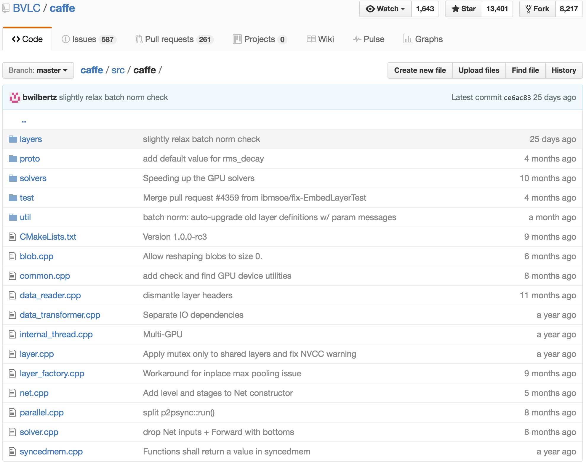
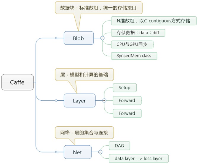
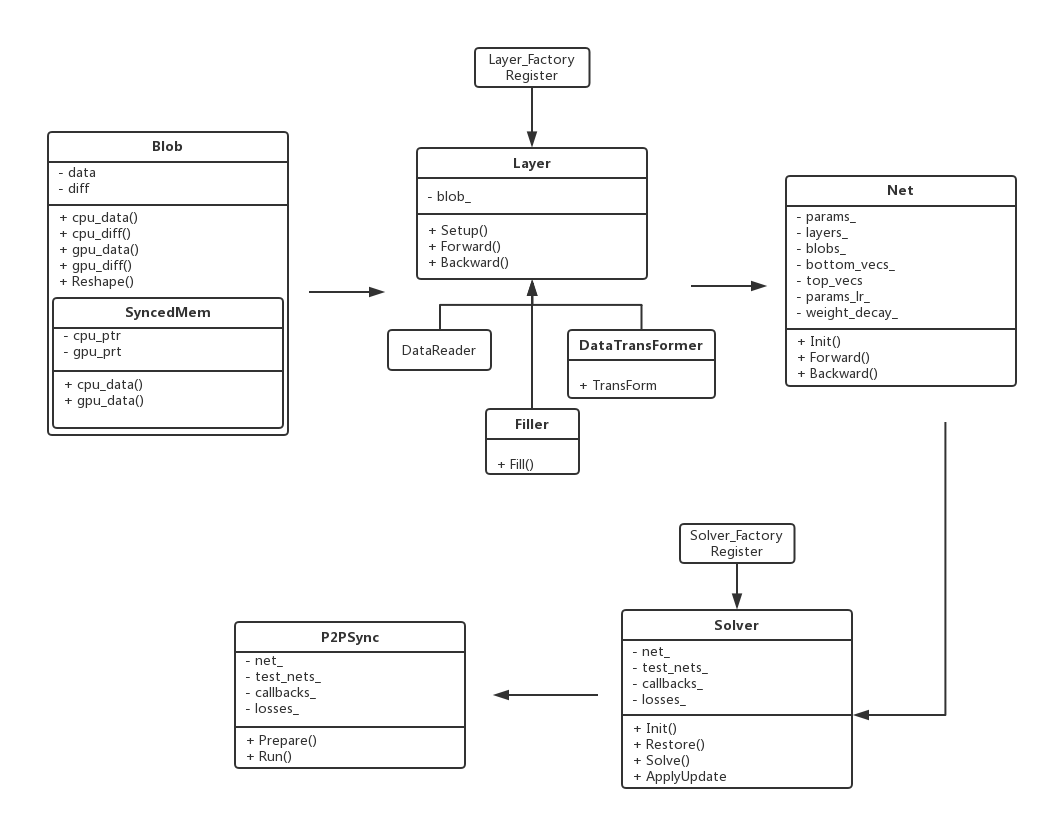
在很多地方都可以看到介绍说caffe种贯穿始终的是Blob,Layer,Net,Solver这几个大类。这四个大类分别负责数据传输、网络层次、网络骨架与参数求解策略,呈现一个自下而上,环环相扣的状态。在源码中可以找到对应这些名称的实现,详细说来,这4个部分分别负责:

Blob:是数据传输的媒介,神经网络涉及到的输入输出数据,网络权重参数等等,其实都是转化为Blob数据结构来存储的。
Layer:是神经网络的基础单元,层与层间的数据节点、前后传递都在该数据结构中被实现,因神经网络网络中设计到多种层,这里layers下实现了卷积层、激励层,池化层,全连接层等等“积木元件”,丰富度很高。
Net:是网络的整体搭建骨架,整合Layer中的层级机构组成网络。
Solver:是网络的求解优化策略,让你用各种“积木”搭建的网络能最适应当前的场景下的样本,如果做深度学习优化研究的话,可能会修改这个模块。

2.2 源码主线结构图

caffe代码的一个精简源码主线结构图如下:

五、caffe项目

5.1 utils

5.2 blob

5.3 Net类

5.4 layers

5.4.1 基本参数

5.4.1.1 proto参数

// Update the next available ID when you add a new LayerParameter field.
// LayerParameter next available layer-specific ID: 149 (last added: clip_param)
message LayerParameter {
    optional string name = 1;   // the layer name
    optional string type = 2;   // the layer type
    repeated string bottom = 3; // the name of each bottom blob
    repeated string top = 4;    // the name of each top blob

    // The train/test phase for computation.
    optional Phase phase = 10;

    // The amount of weight to assign each top blob in the objective.
    // Each layer assigns a default value, usually of either 0 or 1, to each top blob.
    repeated float loss_weight = 5;

    // Specifies training parameters (multipliers on global learning constants,
    // and the name and other settings used for weight sharing).
    repeated ParamSpec param = 6;

    // The blobs containing the numeric parameters of the layer.
    repeated BlobProto blobs = 7;

    // Specifies whether to backpropagate to each bottom. If unspecified,
    // Caffe will automatically infer whether each input needs backpropagation
    // to compute parameter gradients. If set to true for some inputs,
    // backpropagation to those inputs is forced; if set false for some inputs,
    // backpropagation to those inputs is skipped.
    //
    // The size must be either 0 or equal to the number of bottoms.
    repeated bool propagate_down = 11;

      // Rules controlling whether and when a layer is included in the network,
      // based on the current NetState.  You may specify a non-zero number of rules
      // to include OR exclude, but not both.  If no include or exclude rules are
      // specified, the layer is always included.  If the current NetState meets
      // ANY (i.e., one or more) of the specified rules, the layer is
      // included/excluded.
      repeated NetStateRule include = 8;
      repeated NetStateRule exclude = 9;

      // Parameters for data pre-processing.
      optional TransformationParameter transform_param = 100;

      // Parameters shared by loss layers.
      optional LossParameter loss_param = 101;

      // Layer type-specific parameters.
      //
      // Note: certain layers may have more than one computational engine
      // for their implementation. These layers include an Engine type and
      // engine parameter for selecting the implementation.
      // The default for the engine is set by the ENGINE switch at compile-time.
      optional AccuracyParameter accuracy_param = 102;
      optional ArgMaxParameter argmax_param = 103;
      optional BatchNormParameter batch_norm_param = 139;
      optional BiasParameter bias_param = 141;
      optional ClipParameter clip_param = 148;
      optional ConcatParameter concat_param = 104;
      optional ContrastiveLossParameter contrastive_loss_param = 105;
      optional ConvolutionParameter convolution_param = 106;
      optional CropParameter crop_param = 144;
      optional DataParameter data_param = 107;
      optional DropoutParameter dropout_param = 108;
      optional DummyDataParameter dummy_data_param = 109;
      optional EltwiseParameter eltwise_param = 110;
      optional ELUParameter elu_param = 140;
      optional EmbedParameter embed_param = 137;
      optional ExpParameter exp_param = 111;
      optional FlattenParameter flatten_param = 135;
      optional HDF5DataParameter hdf5_data_param = 112;
      optional HDF5OutputParameter hdf5_output_param = 113;
      optional HingeLossParameter hinge_loss_param = 114;
      optional ImageDataParameter image_data_param = 115;
      optional InfogainLossParameter infogain_loss_param = 116;
      optional InnerProductParameter inner_product_param = 117;
      optional InputParameter input_param = 143;
      optional LogParameter log_param = 134;
      optional LRNParameter lrn_param = 118;
      optional MemoryDataParameter memory_data_param = 119;
      optional MVNParameter mvn_param = 120;
      optional ParameterParameter parameter_param = 145;
      optional PoolingParameter pooling_param = 121;
      optional PowerParameter power_param = 122;
      optional PReLUParameter prelu_param = 131;
      optional PythonParameter python_param = 130;
      optional RecurrentParameter recurrent_param = 146;
      optional ReductionParameter reduction_param = 136;
      optional ReLUParameter relu_param = 123;
      optional ReshapeParameter reshape_param = 133;
      optional ScaleParameter scale_param = 142;
      optional SigmoidParameter sigmoid_param = 124;
      optional SoftmaxParameter softmax_param = 125;
      optional SPPParameter spp_param = 132;
      optional SliceParameter slice_param = 126;
      optional SwishParameter swish_param = 147;
      optional TanHParameter tanh_param = 127;
      optional ThresholdParameter threshold_param = 128;
      optional TileParameter tile_param = 138;
      optional WindowDataParameter window_data_param = 129;
}

5.4.2 conv_layer相关文件

5.4.2.2 conv_layer.h文件

5.4.4 batch_norm_layer相关文件

5.4.4.1 proto参数

message BatchNormParameter {
    // If false, normalization is performed over the current mini-batch
    // and global statistics are accumulated (but not yet used) by a moving
    // average.
    // If true, those accumulated mean and variance values are used for the
    // normalization.
    // By default, it is set to false when the network is in the training
    // phase and true when the network is in the testing phase.
    optional bool use_global_stats = 1;
    // What fraction of the moving average remains each iteration?
    // Smaller values make the moving average decay faster, giving more
    // weight to the recent values.
    // Each iteration updates the moving average @f$S_{t-1}@f$ with the
    // current mean @f$ Y_t @f$ by
    // @f$ S_t = (1-\beta)Y_t + \beta \cdot S_{t-1} @f$, where @f$ \beta @f$
    // is the moving_average_fraction parameter.
    optional float moving_average_fraction = 2 [default = .999];
    // Small value to add to the variance estimate so that we don't divide by zero.
  optional float eps = 3 [default = 1e-5];
}

2.4 代码细节

2.4.2 Blob类

前面说到了Blob是最基础的数据结构,用来保存网络传输过程中产生的数据和学习到的一些参数。比如它的上一层Layer中会用下面的形式表示学习到的参数:vector<shared_ptr<Blob<Dtype> > > blobs_;里面的blob就是这里定义的类。部分代码如下:

template <typename Dtype>
class Blob {
 public:
  Blob()
       : data_(), diff_(), count_(0), capacity_(0) {}

  /// @brief Deprecated; use <code>Blob(const vector<int>& shape)</code>.
  explicit Blob(const int num, const int channels, const int height, const int width);
  explicit Blob(const vector<int>& shape);

  /// @brief Deprecated; use <code>Reshape(const vector<int>& shape)</code>.
  void Reshape(const int num, const int channels, const int height,
      const int width);
...

其中template <typename Dtype>表示函数模板,Dtype可以表示int,double等数据类型。Blob是四维连续数组(4-D contiguous array, type = float32), 如果使用(n, k, h, w)表示的话,那么每一维的意思分别是:

n: number. 输入数据量,比如进行sgd时候的mini-batch大小。
c: channel. 如果是图像数据的话可以认为是通道数量。
h,w: height, width. 如果是图像数据的话可以认为是图片的高度和宽度。

实际Blob在(n, k, h, w)位置的值物理位置为((n * K + k) * H + h) * W + w。

Blob内部有两个字段data和diff。Data表示流动数据(输出数据),而diff则存储BP的梯度。

关于blob引入的头文件可以参考下面说明做理解:

#include “caffe/common.hpp”单例化caffe类,并且封装了boost和cuda随机数生成的函数,提供了统一接口。
#include “caffe/proto/caffe.pb.h”上一节提到的头文件
#include “caffe/syncedmem.hpp”主要是分配内存和释放内存的。而class SyncedMemory定义了内存分配管理和CPU与GPU之间同步的函数。Blob会使用SyncedMem自动决定什么时候去copy data以提高运行效率,通常情况是仅当gnu或cpu修改后有copy操作。
#include “caffe/util/math_functions.hpp”封装了很多cblas矩阵运算,基本是矩阵和向量的处理函数。

关于Blob里定义的函数的简单说明如下:

# 构造函数
Blob():data_(), diff_(), count_(0), capacity_(0) {}
explicit Blob(const int num, const int channels, const int height, const int width);
explicit Blob(const vector<int>& shape);

# Reshape函数:改变一个blob的大小
void Reshape(const int num, const int channels, const int height,const int width);
void Reshape(const vector<int>& shape);
void Reshape(const BlobShape& shape);

inline int num() const { return LegacyShape(0); }
inline int channels() const { return LegacyShape(1); }
inline int height() const { return LegacyShape(2); }
inline int width() const { return LegacyShape(3); }


# ReshapeLike函数:为data和diff重新分配一块空间,大小和另一个blob的一样
void ReshapeLike(const Blob& other);

# shape_string函数:打印blob shape
inline string shape_string() const

# shape函数:返回blob的shape或者指定位置shape大小
inline const vector<int>& shape() const { return shape_; }
inline int shape(int index) const {return shape_[CanonicalAxisIndex(index)];}

# num_axes函数:返回blob的大小
inline int num_axes() const { return shape_.size(); }

# count函数:返回指定位置的元素数量
inline int count() const { return count_; }
inline int count(int start_axis, int end_axis) const;
inline int count(int start_axis) const {} // count(start_axis, num_axes())

# offset函数:得到blob数据的偏移位置
inline int offset(const int n, const int c = 0, const int h = 0,const int w = 0) const
inline int offset(const vector<int>& indices) const

# CopyFrom函数:从source拷贝数据,copy_diff来作为标志区分是拷贝data还是diff
void CopyFrom(const Blob<Dtype>& source, bool copy_diff = false,bool reshape = false);

# 获取数据相关的函数
inline Dtype data_at(const int n, const int c, const int h,const int w) const { return cpu_data()[offset(n, c, h, w)]; }
inline Dtype diff_at(const int n, const int c, const int h, const int w) const { return cpu_diff()[offset(n, c, h, w)]; }
inline Dtype data_at(const vector<int>& index) const { return cpu_data()[offset(index)]; }
inline Dtype diff_at(const vector<int>& index) const { return cpu_diff()[offset(index)]; }

inline const shared_ptr<SyncedMemory>& data() const { CHECK(data_); return data_; }
inline const shared_ptr<SyncedMemory>& diff() const { CHECK(diff_); return diff_; }

const Dtype* cpu_data() const;
void set_cpu_data(Dtype* data);
const int* gpu_shape() const;
const Dtype* gpu_data() const;
void set_gpu_data(Dtype* data);
const Dtype* cpu_diff() const;
const Dtype* gpu_diff() const;
Dtype* mutable_cpu_data();
Dtype* mutable_gpu_data();
Dtype* mutable_cpu_diff();
Dtype* mutable_gpu_diff();


# blob相关计算的函数
Dtype asum_data() const; // L1 norm
Dtype asum_diff() const; // L1 norm

Dtype sumsq_data() const; // L2 norm
Dtype sumsq_diff() const; // L2 norm

void scale_data(Dtype scale_factor); // 点乘
void scale_diff(Dtype scale_factor); // 点乘


# FromProto函数:从proto读数据进来,其实就是反序列化
void FromProto(const BlobProto& proto, bool reshape = true);

# ToProto函数: 把blob数据保存到proto中
void ToProto(BlobProto* proto, bool write_diff = false) const;


void Update();

# ShareDate/ShareDiff函数: 从other的blob复制data和diff的值;
void ShareData(const Blob& other);
void ShareDiff(const Blob& other);

# ShapeEquals:判断是否与指定的blob shape相同
bool ShapeEquals(const BlobProto& other);

# 相关保护变量
shared_ptr<SyncedMemory> data_;
shared_ptr<SyncedMemory> diff_;
shared_ptr<SyncedMemory> shape_data_;
vector<int> shape_;
int count_;
int capacity_;

2.4.3 Layer类

Layer是网络的基本单元(“积木”),由此派生出了各种层类。如果做数据特征表达相关的研究,需要修改这部分。Layer类派生出来的层类通过这实现两个虚函数Forward()和Backward(),产生了各种功能的层类。Forward是从根据bottom计算top的过程,Backward则刚好相反。在网路结构定义文件(*.proto)中每一层的参数bottom和top数目就决定了vector中元素数目。

一起来看看Layer.hpp

#include <algorithm>
#include <string>
#include <vector>

#include "caffe/blob.hpp"
#include "caffe/common.hpp"
#include "caffe/layer_factory.hpp"
#include "caffe/proto/caffe.pb.h"
#include "caffe/util/math_functions.hpp"

/**
 Forward declare boost::thread instead of including boost/thread.hpp
 to avoid a boost/NVCC issues (#1009, #1010) on OSX.
 */
namespace boost { class mutex; }

namespace caffe {
...
template <typename Dtype>
class Layer {
 public:
  /**
   * You should not implement your own constructor. Any set up code should go
   * to SetUp(), where the dimensions of the bottom blobs are provided to the
   * layer.
   */
  explicit Layer(const LayerParameter& param)
    : layer_param_(param), is_shared_(false) {
      // Set phase and copy blobs (if there are any).
      phase_ = param.phase();
      if (layer_param_.blobs_size() > 0) {
        blobs_.resize(layer_param_.blobs_size());
        for (int i = 0; i < layer_param_.blobs_size(); ++i) {
          blobs_[i].reset(new Blob<Dtype>());
          blobs_[i]->FromProto(layer_param_.blobs(i));
        }
      }
    }
  virtual ~Layer() {}
...

Layer中三个重要参数:

LayerParameter layer_param_:表示protobuf文件中存储的layer参数。
Phase phase_:表示网络的级别(TRAIN/TEST)
vector<share_ptr<Blob<Dtype>>> blobs_:表示存储的是layer学习到的参数。
vector<bool> param_propagate_down_:表示是否计算各个blob参数的diff,即传播误差。

包含了一些基本函数:

# 构造函数(基本上从protobuf读取参数)
explicit Layer(const LayerParameter& param);
virtual ~Layer();

# 对参数进行格式化
void SetUp(const vector<Blob<Dtype>*>& bottom, const vector<Blob<Dtype>*>& top)


# 核心计算(输入统一都是 bottom,输出为top,其中Backward里面有个propagate_down参数, 用来表示该Layer是否反向传播参数)
inline Dtype Forward(const vector<Blob<Dtype>*>& bottom, const vector<Blob<Dtype>*>& top);     # 前向计算
inline void Backward(const vector<Blob<Dtype>*>& top, const vector<bool>& propagate_down, const vector<Blob<Dtype>*>& bottom); # 后向更新

2.4.4 Net类

Net是网络的搭建部分,将Layer所派生出层类组合成网络。 Net用容器的形式将多个Layer有序地放在一起,它自己的基本功能主要是对逐层Layer进行初始化,以及提供Update()的接口用于更新网络参数, 本身不能对参数进行有效地学习过程。

vector<shared_ptr<Layer<Dtype> > > layers_;

Net也有它自己的Forward()和Backward(),他们是对整个网络的前向和反向传导,调用可以计算出网络的loss。Net由一系列的Layer组成(无回路有向图DAG),Layer之间的连接由一个文本文件描述。模型初始化Net::Init()会产生blob和layer并调用Layer::SetUp。在此过程中Net会报告初始化进程。这里的初始化与设备无关,在初始化之后通过Caffe::set_mode()设置Caffe::mode()来选择运行平台CPU或 GPU,结果是相同的。

solver优化

常用的优化方法

SGD

此处的SGD指mini-batch gradient descent,关于batch gradient descent, stochastic gradient descent, 以及 mini-batch gradient descent的具体区别就不细说了。现在的SGD一般都指mini-batch gradient descent。

SGD就是每一次迭代计算mini-batch的梯度,然后对参数进行更新,是最常见的优化方法了。即:

$\begin{aligned} & g_t=\nabla_{\theta_{t-1}}f(\theta_{t-1}) \\ & \theta_t=\theta_{t-1}-\eta * g_t \end{aligned}$

其中, $\eta$ 是学习率, $g_t$ 是梯度 SGD完全依赖于当前batch的梯度,所以 $\eta$ 可理解为允许当前batch的梯度多大程度影响参数更新

缺点:

选择合适的learning rate比较困难 - 对所有的参数更新使用同样的learning rate。对于稀疏数据或者特征,有时我们可能想更新快一些对于不经常出现的特征,对于常出现的特征更新慢一些,这时候SGD就不太能满足要求了

SGD容易收敛到局部最优,并且在某些情况下可能被困在鞍点【原来写的是“容易困于鞍点”,经查阅论文发现,其实在合适的初始化和step size的情况下,鞍点的影响并没这么大。感谢@冰橙的指正】

Momentum momentum是模拟物理里动量的概念,积累之前的动量来替代真正的梯度。公式如下:

$\begin{aligned} & m_t=\mu * m_{t-1}+g_t \\ & \theta_t=\theta_{t-1}-\eta * m_t \end{aligned}$

其中, $\mu$ 是动量因子

特点:

下降初期时,使用上一次参数更新,下降方向一致,乘上较大的[公式]能够进行很好的加速

下降中后期时,在局部最小值来回震荡的时候, $gradient\rightarrow 0,\mu$ 使得更新幅度增大,跳出陷阱

在梯度改变方向的时候, $\mu$ 能够减少更新总而言之,momentum项能够在相关方向加速SGD,抑制振荡,从而加快收敛

Nesterov

nesterov项在梯度更新时做一个校正,避免前进太快,同时提高灵敏度。将上一节中的公式展开可得:

$\theta_t=\theta_{t-1}-\eta * \mu * m_{t-1}-\eta * g_t$

可以看出, $m_{t-1}$ 并没有直接改变当前梯度 $g_t$ ,所以Nesterov的改进就是让之前的动量直接影响当前的动量。即:

$\begin{aligned} & g_t = \nabla_{\theta_{t-1}}f(\theta_{t-1}-\eta * \mu * m_{t-1}) \\ & m_t = \mu * m_{t-1} + g_t \\ & \theta_t = \theta_{t-1}-\eta * m_t \end{aligned}$

所以,加上nesterov项后,梯度在大的跳跃后,进行计算对当前梯度进行校正。如下图:

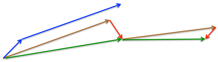
momentum首先计算一个梯度(短的蓝色向量),然后在加速更新梯度的方向进行一个大的跳跃(长的蓝色向量),nesterov项首先在之前加速的梯度方向进行一个大的跳跃(棕色向量),计算梯度然后进行校正(绿色梯向量)

其实,momentum项和nesterov项都是为了使梯度更新更加灵活,对不同情况有针对性。但是,人工设置一些学习率总还是有些生硬,接下来介绍几种自适应学习率的方法

Adagrad

Adagrad其实是对学习率进行了一个约束。即:

$\begin{aligned} & n_t = n_{t-1} + g_t^2 \\ & \Delta \theta_t = -\frac{\eta}{\sqrt{n_t+\epsilon}} * g_t \end{aligned}$

此处,对 $g_t$ 从1到 $t$ 进行一个递推形成一个约束项regularizer, $-\frac{1}{\sqrt{\sum_{r=1}^t(g_t)^2+\epsilon}},\epsilon$ 用来保证分母非0

特点:

前期 $g_t$ 较小的时候, regularizer较大,能够放大梯度

后期 $g_t$ 较大的时候,regularizer较小,能够约束梯度

适合处理稀疏梯度

缺点:

由公式可以看出,仍依赖于人工设置一个全局学习率

$\eta$ 设置过大的话,会使regularizer过于敏感,对梯度的调节太大

中后期,分母上梯度平方的累加将会越来越大,使 $gradient\rightarrow 0$ ,使得训练提前结束

Adadelta

Adadelta是对Adagrad的扩展,最初方案依然是对学习率进行自适应约束,但是进行了计算上的简化。 Adagrad会累加之前所有的梯度平方,而Adadelta只累加固定大小的项,并且也不直接存储这些项,仅仅是近似计算对应的平均值。即:

$\begin{aligned} & n_t=\upsilon * n_{t-1}+(1-\upsilon)*g_t \\ & \Delta \theta_t=-\frac{\eta}{\sqrt{n_t+\epsilon}} * g_t \end{aligned}$

在此处Adadelta其实还是依赖于全局学习率的,但是作者做了一定处理,经过近似牛顿迭代法之后:

$\begin{aligned} & E|g^2|_t = \rho * E|g^2|_{t-1}+(1-\rho)*g_t^2 \\ & \Delta x_t=\frac{\sqrt{\sum_{r=1}^{t-1}\Delta x_r}}{\sqrt{E|g^2|_t+\epsilon}} \end{aligned}$

其中, $E$ 代表求期望。此时,可以看出Adadelta已经不用依赖于全局学习率了。

特点:

训练初中期,加速效果不错,很快

训练后期,反复在局部最小值附近抖动

RMSprop

RMSprop可以算作Adadelta的一个特例:当 $\rho=0.5$ 时, $E|g^2|_t=\rho * E|g^2|_{t-1} + (1-\rho) * g_t^2$ 就变为了求梯度平方和的平均数。

如果再求根的话,就变成了RMS(均方根):

$RMS|g|_t = \sqrt{E|g^2|_t+\epsilon}$

此时,这个RMS就可以作为学习率[公式]的一个约束:

$\Delta x_t=-\frac{\eta}{EMS|g|_t} * g_t$

特点:

其实RMSprop依然依赖于全局学习率

RMSprop算是Adagrad的一种发展,和Adadelta的变体,效果趋于二者之间

适合处理非平稳目标 - 对于RNN效果很好

Adam

Adam(Adaptive Moment Estimation)本质上是带有动量项的RMSprop,它利用梯度的一阶矩估计和二阶矩估计动态调整每个参数的学习率。Adam的优点主要在于经过偏置校正后,每一次迭代学习率都有个确定范围,使得参数比较平稳。公式如下:

$\begin{aligned} & m_t = \mu * m_{t-1} + (1-\mu)*g_t \\ & n_t = \upsilon * n_{t-1} + (1-\upsilon) * g_t^2 \\ & \hat{m_t} = \frac{m_t}{1-\mu^t} \\ & \hat{n_t} = \frac{n_t}{1-\upsilon^t} \\ & \Delta\theta_t = -\frac{\hat{m_t}}{\sqrt{\hat{n_t}}+\epsilon} * \eta \end{aligned}$

其中, $m_t,n_t$ 分别是对梯度的一阶矩估计和二阶矩估计,可以看作对期望 $E|g_t|,E|g^2_t|$ 的估计; $\hat{m}_t,\hat{n}_t$ 是对 $m_t,n_t$ 的校正,这样可以近似为对期望的无偏估计。可以看出,直接对梯度的矩估计对内存没有额外的要求,而且可以根据梯度进行动态调整,而[公式]对学习率形成一个动态约束,而且有明确的范围。

特点:

结合了Adagrad善于处理稀疏梯度和RMSprop善于处理非平稳目标的优点

对内存需求较小

为不同的参数计算不同的自适应学习率

也适用于大多非凸优化 - 适用于大数据集和高维空间

Adamax

Adamax是Adam的一种变体,此方法对学习率的上限提供了一个更简单的范围。公式上的变化如下:

$\begin{aligned} & n_t = max(\upsilon * n_{t-1}, |g_t|) \\ & \Delta x = -\frac{\hat{m}_t}{n_t+\epsilon} * \eta \end{aligned}$

可以看出,Adamax学习率的边界范围更简单

Nadam

Nadam类似于带有Nesterov动量项的Adam。公式如下:

$\begin{aligned} & \hat{g}_t=\frac{g_t}{1-\prod_{i=1}^t\mu_i} \\ & m_t = \mu_t * m_{t-1} + (1-\mu_t)*g_t \\ & \hat{m}_t=\frac{m_t}{1-\prod_{i=1}^{t+1}\mu_i} \\ & n_t = \upsilon * n_{t-1} + (1-\upsilon)*g_t^2 \\ & \hat{n}_t = \frac{n_t}{1-\upsilon^t} \\ & \bar{m}_t = (1-\mu_t) * \hat{g}_t + \mu_{t+1} * \hat{m}_t \\ & \Delta \theta_t = - \eta * \frac{\hat{m}_t}{\sqrt{\hat{n}_t} + \epsilon} \end{aligned}$

可以看出,Nadam对学习率有了更强的约束,同时对梯度的更新也有更直接的影响。一般而言,在想使用带动量的RMSprop,或者Adam的地方,大多可以使用Nadam取得更好的效果。

经验之谈

对于稀疏数据,尽量使用学习率可自适应的优化方法,不用手动调节,而且最好采用默认值

SGD通常训练时间更长,但是在好的初始化和学习率调度方案的情况下,结果更可靠

如果在意更快的收敛,并且需要训练较深较复杂的网络时,推荐使用学习率自适应的优化方法。

Adadelta,RMSprop,Adam是比较相近的算法,在相似的情况下表现差不多。

在想使用带动量的RMSprop,或者Adam的地方,大多可以使用Nadam取得更好的效果

// 这个枚举类型定义获得外界信号的几种定义
namespace SolverAction {
    enum Enum {
        NONE = 0,  // 忽略信号什么都不做
        STOP = 1,  // 停止训练
        SNAPSHOT = 2  // 保存快照,继续训练
    };
}

// 定义信号回调函数
typedef boost::function<SolverAction::Enum()> ActionCallback;


template <typename Dtype>
class Solver {
    public:
        explicit Solver(const SolverParameter& param);
        explicit Solver(const string& param_file);
        void Init(const SolverParameter& param);
        void InitTrainNet();
        void InitTestNets();

  // Client of the Solver optionally may call this in order to set the function
  // that the solver uses to see what action it should take (e.g. snapshot or
  // exit training early).
  void SetActionFunction(ActionCallback func);
  SolverAction::Enum GetRequestedAction();
  // The main entry of the solver function. In default, iter will be zero. Pass
  // in a non-zero iter number to resume training for a pre-trained net.
  virtual void Solve(const char* resume_file = NULL);
  inline void Solve(const string& resume_file) { Solve(resume_file.c_str()); }
  void Step(int iters);
  // The Restore method simply dispatches to one of the
  // RestoreSolverStateFrom___ protected methods. You should implement these
  // methods to restore the state from the appropriate snapshot type.
  void Restore(const char* resume_file);
  // The Solver::Snapshot function implements the basic snapshotting utility
  // that stores the learned net. You should implement the SnapshotSolverState()
  // function that produces a SolverState protocol buffer that needs to be
  // written to disk together with the learned net.
  void Snapshot();
  virtual ~Solver() {}
  inline const SolverParameter& param() const { return param_; }
  inline shared_ptr<Net<Dtype> > net() { return net_; }
  inline const vector<shared_ptr<Net<Dtype> > >& test_nets() {
    return test_nets_;
  }
  int iter() const { return iter_; }

  // Invoked at specific points during an iteration
  class Callback {
   protected:
    virtual void on_start() = 0;
    virtual void on_gradients_ready() = 0;

    template <typename T>
    friend class Solver;
  };
  const vector<Callback*>& callbacks() const { return callbacks_; }
  void add_callback(Callback* value) {
    callbacks_.push_back(value);
  }

  void CheckSnapshotWritePermissions();
  /**
   * @brief Returns the solver type.
   */
  virtual inline const char* type() const { return ""; }

  // Make and apply the update value for the current iteration.
  virtual void ApplyUpdate() = 0;

 protected:
  string SnapshotFilename(const string& extension);
  string SnapshotToBinaryProto();
  string SnapshotToHDF5();
  // The test routine
  void TestAll();
  void Test(const int test_net_id = 0);
  virtual void SnapshotSolverState(const string& model_filename) = 0;
  virtual void RestoreSolverStateFromHDF5(const string& state_file) = 0;
  virtual void RestoreSolverStateFromBinaryProto(const string& state_file) = 0;
  void DisplayOutputBlobs(const int net_id);
  void UpdateSmoothedLoss(Dtype loss, int start_iter, int average_loss);

  SolverParameter param_;
  int iter_;
  int current_step_;
  shared_ptr<Net<Dtype> > net_;
  vector<shared_ptr<Net<Dtype> > > test_nets_;
  vector<Callback*> callbacks_;
  vector<Dtype> losses_;
  Dtype smoothed_loss_;

  // A function that can be set by a client of the Solver to provide indication
  // that it wants a snapshot saved and/or to exit early.
  ActionCallback action_request_function_;

  // True iff a request to stop early was received.
  bool requested_early_exit_;

  // Timing information, handy to tune e.g. nbr of GPUs
  Timer iteration_timer_;
  float iterations_last_;

  DISABLE_COPY_AND_ASSIGN(Solver);
};

}  // namespace caffe

#endif  // CAFFE_SOLVER_HPP_

template <typename Dtype>
class Solver {
    public:
        // 构造函数
        explicit Solver(const SolverParameter& param);
        explicit Solver(const string& param_file);
        // 初始化类和训练测试网络
        void Init(const SolverParameter& param);
        void InitTrainNet();
        void InitTestNets();

        // 传入信号传递函数指针(如何处理信号)
        void SetActionFunction(ActionCallback func);
        // 返回信号
        SolverAction::Enum GetRequestedAction();
  // The main entry of the solver function. In default, iter will be zero. Pass
  // in a non-zero iter number to resume training for a pre-trained net.
        // 训练的主函数(多次Step函数)
        virtual void Solve(const char* resume_file = NULL);
        inline void Solve(const string& resume_file) { Solve(resume_file.c_str()); }
        // 每一步的迭代函数
        void Step(int iters);

        // 存储函数实现如何存储solver到快照模型中
        void Restore(const char* resume_file);

        // 主要是基本的快照功能,存储学习的网络
        void Snapshot();
        virtual ~Solver() {}
        // 返回配置参数变量
        inline const SolverParameter& param() const { return param_; }
        // 返回网络指针
        inline shared_ptr<Net<Dtype> > net() { return net_; }
        // 返回测试网络指针
        inline const vector<shared_ptr<Net<Dtype> > >& test_nets() { return test_nets_; }
        // 返回迭代次数
        int iter() const { return iter_; }

        // 在迭代过程中在指定点执行的回调函数
        class Callback {
            protected:
                virtual void on_start() = 0;
                virtual void on_gradients_ready() = 0;

                template <typename T>
                friend class Solver;
        };
        const vector<Callback*>& callbacks() const { return callbacks_; }
        void add_callback(Callback* value) { callbacks_.push_back(value); }

        // 检查快照写的权限
        void CheckSnapshotWritePermissions();

        // 返回solver type
        virtual inline const char* type() const { return ""; }

        // 在当前迭代过程中执行更新
        virtual void ApplyUpdate() = 0;

    protected:
        string SnapshotFilename(const string& extension);
        string SnapshotToBinaryProto();
        string SnapshotToHDF5();

        // 测试
        void TestAll();
        void Test(const int test_net_id = 0);
  virtual void SnapshotSolverState(const string& model_filename) = 0;
  virtual void RestoreSolverStateFromHDF5(const string& state_file) = 0;
  virtual void RestoreSolverStateFromBinaryProto(const string& state_file) = 0;
  void DisplayOutputBlobs(const int net_id);
  void UpdateSmoothedLoss(Dtype loss, int start_iter, int average_loss);

        SolverParameter param_;
        int iter_;      // 迭代次数
        int current_step_;  // 当前迭代次数
        shared_ptr<Net<Dtype> > net_; // 网络指针
        vector<shared_ptr<Net<Dtype> > > test_nets_; // 测试网络指针
        vector<Callback*> callbacks_; // 回调函数
        vector<Dtype> losses_;        // loss变量
        Dtype smoothed_loss_;

        ActionCallback action_request_function_;

  // True iff a request to stop early was received.
  bool requested_early_exit_;

  // Timing information, handy to tune e.g. nbr of GPUs
  Timer iteration_timer_;
  float iterations_last_;

  DISABLE_COPY_AND_ASSIGN(Solver);
};