摆线知识

圆形是我们学习数学以来最先接触的特殊图形——它没法被分解成有限个三角形。我们如果在一个滚轮的边上一定点放置一支笔,然后让滚轮沿着墙壁滚动,就能够在墙上画出摆线(Cycloid)的图像:

不妨再用几何的方法来得到其参数方程:

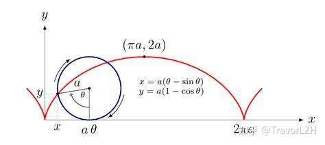
经过一定的分析，我们最终可以得到一组方程来描述摆线(其中a为圆的半径):

一、摆线的基本性质

根据三角函数的性质以及摆线的绘制过程,我们知道$0\le\theta\le2\pi$内(即滚轮旋转一周)的曲线构成摆线的一个弧。所以我们可以根据这个性质来求出摆线一个周期的弧长。

第一步:计算弧微分

根据勾股定理$(\mathrm{d}s)^2=(\mathrm{d}x)^2+(\mathrm{d}y)^2$,我们得到:

由于我们$\theta$的取值范围内正弦函数不会取负值,因此我们可以放心的去掉绝对值符号。

第二步:计算曲线积分

因此,一个滚轮转动一周形成摆线的弧长刚好是滚轮半径的八倍。

二、最速降线问题

最速降线问题,即找到两个定点间连接的曲线,使得物体能够在重力作用下花最短的时间到达终点。早在1696年,著名数学家约翰·伯努利(Johann Bernoulli)就提出了这个问题。当时欧洲各地的数学家都使用了不同的方法来求解这个问题。然而,伯努利本人提出这个挑战的初衷是为了凸显自己方法的高明从而体现他自己很聪明。他本人花了近两个星期找到这个方法。然而他向欧洲发表这个问题后仅仅一天,已经退休牛顿就给出了他的解法。牛顿在后来的书信里曾说道:"我不喜欢让外国人嘲弄我的数学能力"。后来,伯努利的学生欧拉(Leonard Euler)不仅给出了最速降线问题的另一种解法,还设计了欧拉—拉格朗日方程(Euler—Lagrange equation)来解决类似的问题。本节中我将着重讲述伯努利和欧拉的解法。

• 费马原理与斯涅尔定律

在直接进入最速降线问题的推导前,我们需要提及费马原理(Fermat's principle),即在两点间,光总是选择耗时最短的路径。利用这个原理,我们可以研究一下光的折射性质:

现在我们想研究一下入射角与折射角的关系。不同于求证光的反射定律,我们需要用上述的费马原理来求解$\alpha$与$\beta$的关系。假设光在白色区域内的传播速度为$v_1$,而它在蓝色区域的传播速度为$v_2$,现在我们要找到合适的$x$,使得光沿着红色路线的传播时间最少(即找到最快传播路径)。

本篇文章将使用微积分里优化函数的方法来求解。根据勾股定理,我们不难得出:

现在,我们再列出要优化的时间函数:

现在对$x$求导,得到:

我们知道,当导数为0或未定义时,函数取极值。然而在在T函数的定义域内,函数只在导数为0时达到最小值。因此,我们能够列出这样的方程来求解$x$:

根据原图,我们不难得出$\sin\alpha={x\over\sqrt{x^2+a^2}}$,$\cos\alpha={d-x\over\sqrt{(d-x)^2+b^2}}$。因此,代入到原式,我们就得到了入射角$\alpha$与折射角$\beta$的关系:

因此,入射角与折射角的正弦比刚好等于两种介质下的光速比,这个结论又叫做斯涅尔定律(Snell's law)。虽然斯涅尔定律是一个光学定律,但是在力学中它依然适用。

三、伯努利解法——用斯涅尔定律求解最速降线

我们设物体最初距离地面的高度为$h$,而物体的当前速度和高度分别为$v=v(t)$和$y=y(t)$。根据(理想状态下)机械能守恒,我们可以对物体的速度和当前高度建立如下关系:

由于物体的质量恒不为0,所以我们可以直接让等式两侧与之相除:

根据基本代数操作,我们不难得出物体速度关于其纵坐标的表达式:

根据幂函数的性质,物体的纵坐标其速度一一对应。如果我们把每个纵坐标都当作一个不同的介质而每个不同的介质下的光速都为$\sqrt{2g(h-y)}$,我们可以把最速降线问题理解成光在多个不同介质下的传播问题。根据费马原理,光总是沿着耗时最短的路径传播,所以我们如果用光学的原则求解出耗时最短的传播路径,就可以得到最速降线问题的答案。

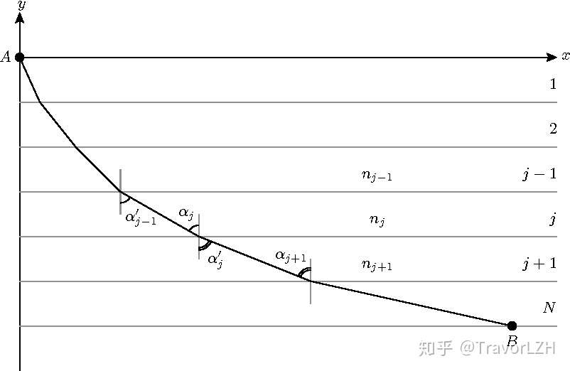
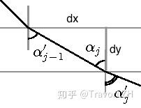
如果我们把物体的运动空间用平行于x轴的直线进行分割,就可以发现当"光线"从第j个区间穿越到第j+1个区间进行折射时,折射角满足斯涅尔定律。因此:

由于我们所做的发现均垂直于x轴(即平行于y轴),所以这些法线都相互平行。于是,根据两直线平行,内错角相等的原则,我们得到$\alpha'_j=\alpha_{j+1}$,因此,我们可以把上述等式进行这样的拓展:

因此每一个区间内入射角的正弦于区间内的传播速度成正比,而比例常数设为C。因此,我们可以再把速度关于y的表达式代入,得到:

经过一定代数操作,我们可以得到y关于$\sin\alpha$的表达式:

现在我们再来看一看入射角于物体坐标微小变化的关系:

我们不难发现${\mathrm{d}x\over\mathrm{d}y}=\tan\alpha$,因此我们可以通过$\alpha$构造一个最速降线的参数方程。现在我们先让y对$\alpha$求导,得到下式:

根据链式法则,我们可以得到x关于$\alpha$的微分方程:

现在两侧积分,我们可以得到:

现在我们可以将y的表达式改写,得到:

为了美观,我们可以更换自变量$\theta=2\alpha$,得到最速降线最后的参数方程:

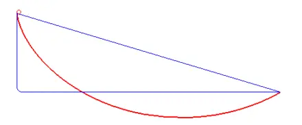
我们不难发现最速降线的参数方程画出的图像刚刚好就是翻转后的摆线:

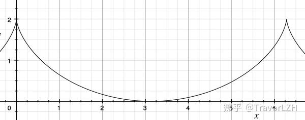
因此,最速降线的答案就是摆线。以上便是伯努利的解法,现在我们再来看看他的学生——欧拉——的解法。

四、欧拉的解法——变分法

我们先来看一下什么是泛函(functional)。泛函一般指从一个空间到数域的映射。

对于一个实变函数$f$,$f\mapsto f(x_0)$就是一个基本的泛函,它把函数空间映射到了实数域。而另外一种常见泛函则由积分构成:

或许读者看到这里会有些摸不着头脑,但是我们这些内容会为后面的求解提供铺垫。现在我们来看一看泛函极值问题:找到一个满足$y(x_0)=y_0,y(x_1)=y_1$的$y$,使得泛函$J[y]=\int_{x_0}^{x_1}F(x,y,y')\mathrm{d}x$取得极值。

在传统的单变量微积分里的优化问题中,我们一般都会通过寻找导数的零点来寻找函数的极值。在泛函里我们会寻找变分(variation)的零点来求得泛函的极值。如果我们假设y就是最终满足泛函达到极值的函数,而$u=y+\eta$表示的是y领域内的函数(其中$\eta(x_0)=\eta(x_1)=0$以便于所有的u满足y的边界条件)。则:

对于足够"微小"的y,我们可以用泛函核$F$在$F(x,y,y')$附近的一阶泰勒展开来"估计"$F(x,y+\eta,y'+\eta)$:

现在我们对被积函数里的第二项进行分部积分,得:

根据$\eta$满足$\eta(x_0)=\eta(x_1)=0$的性质,我们可以得到泛函$J$变分的最简形式:

由于在$J[y]$处取得极值,所以根据"直觉",我们可以得到$\delta J=0$。我们也不难能看出(变分法基本引理),$\delta J=0$当且仅当被积函数里$\eta$的系数在区间内恒为0。因此,我们不严谨地推导出了:

即大名鼎鼎的欧拉—拉格朗日方程(Euler—Lagrange equation),简称E-L方程。知乎有很多其它的推导过程,但是它们大多数都设$u=y+\varepsilon\eta$然后求泛函对$\varepsilon$的全微分。虽然这样更加的严谨,但是作者个人最容易理解的推导还是以上$u=y+\eta$的方法。

虽然E-L方程可以解决大多数泛函极值问题,但是对于满足${\partial F\over\partial x}=0$的泛函,直接代入E-L方程会比较产生比较复杂的微分方程。因此,我们决定再简化一下难度,对E-L方程进行移项:

对两侧乘上y'并积分,得到:

因此,我们可以在优化满足$F=F(y,y')$的泛函使用我们得到的结论,即贝尔特拉米等式(Beltrami's identity)。我们已经将所有需要的工具准备完毕,现在可以开始进入最速降线问题的求解了。

用变分法求解最速降线问题

由于我们要找到一个曲线,使得物体沿曲线路径滑落的时间最短,我们需要设计一个描述时间的泛函:

利用弧微分公式和前面提到的能量守恒,我们不难得出:

因此,我们的得到了这样的时间泛函:

因此,我们的最速降线问题变成变分问题,即找到一个满足边界条件的y,使得泛函T取得极值。由于泛函T的核F满足${\partial F\over\partial x}=0$,所以我们可以使用更加方便的贝尔特拉米等式来求解。首先,我们求F关于y'的偏导数:

代入到贝尔特拉米等式,得到:

此时,我们如果令$y'\equiv{\mathrm{d}y\over\mathrm{d}x}=\cot\alpha$,则根据三角恒等式$\csc^2\alpha=1+\cot^2\alpha$,原式变成:

我们可以发现这个方程和我们用斯涅尔定律得出的方程完全一样,所以其实伯努利和欧拉的方法都能够说明最速降线问题的答案是摆线。然而,摆线的故事才刚刚开始。摆线不仅是最速降线问题的答案,还是等时降落问题(Tautochrone problem)的解。

摆线与等时降落问题——弹簧与硬核的阿贝尔

等时降落问题,即找到一个合适的曲线,使得物体从曲线的任何位置受重力作用(理想状态下无摩擦)滑落到终点的时间不变。

当然,在我们有头绪之前。我们先来研究研究弹簧振子的简单调谐运动(Simple harmonic motion)。其中弹簧振子的位置x满足如下微分方程:

我们设初始条件:$x(0)=x_0,\left.\mathrm{d}x\over\mathrm{d}t\right|_{t=0}=0$,即物体的初速度为0而初始位置为$x_0$。因此,在我们对微分方程进行拉氏变换时能够得到:

根据余弦函数的性质,我们不难发现x的第一个零点在$t={\pi\over2\omega}$,而且这个零点与$x_0$的值无关。这意味着(理想状态下)无论$x_0$多大,${\pi\over2\omega}$秒后x总能回到0。意思就是说无论你把弹簧拉到多长,弹簧总能够在指定时间后回到原点。

利用简谐运动求解等时降落问题

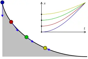
我们引入广义坐标s来描述示意图终点与物体当前位置间曲线的弧长,则根据等时降落曲线满足:s变成0的耗时与$s_0$无关,这意味着s可能会满足简谐运动方程,即:

现在我们在来看看作用在物体上的加速度。

由于蓝色部分的分量刚好被约束抵消,所以物体在曲线上的加速度刚好等于$-g\sin\theta$,因此我们不难发现${\mathrm{d}^2s\over\mathrm{d}t^2}=-g\sin\theta$。再代入到s满足的简谐运动方程,我们得到了等时降落曲线的微分方程:

现在我们对等式两侧两侧微分，则

读者可以根据上图$\theta$以及三角函数本身的定义推出一下面两个式子:

分别将以上两个等式代入到原来的微分方程中,我们可以得到两个方程:

现在对两侧分别进行积分,得到:

以及

依照上面最速降线的传统,我们可以进行换元:$\phi=2\theta$,则我们得到的等时降落曲线方程为:

因此,我们利用简谐运动方程发现(翻转后的)摆线是等时降落问题的答案。这就是等时降落问题的一个传统解法,但是阿贝尔用却能量守恒给出了一个更加硬核的解答。

阿贝尔的硬核解法——积分方程法

与简谐运动方程法一样,阿贝尔也采用了同样的广义坐标s。现在把s代入到机械能守恒方程里(h为物体初始位置的纵坐标),得到(符号是因为物体下滑时s单调递减):

根据问题的定义,我们知道等时降落问题的曲线满足物体降落时间与出发位置无关,即曲线满足$\int_{y=h}^{y=0}\mathrm{d}t=T$(T为常数)。利用链式法则,我们发现$\mathrm{d}t={\mathrm{d}t\over\mathrm{d}s}{\mathrm{d}s\over\mathrm{d}y}\mathrm{d}y=-{1\over\sqrt{2g}\sqrt{h-y}}{\mathrm{d}s\over\mathrm{d}y}\mathrm{d}y$,所以最后代入到原来的积分式,得到:

于是我们得到了著名的阿贝尔积分方程(Abel integral equation)。在上一篇文章里,我使用分数阶微积分的方法求解了这个方程,但这次我打算使用拉普拉斯变换来求解:

我们不难发现等式右侧刚好是一个卷积,因此根据卷积定理(Convolution theorem),右侧可以改写成两个拉氏变换的乘积:

$<span><span class="MathJax_Preview">\mathcal{L}\{\sqrt{2g}T\}=\mathcal{L}\{y^{-1/2}\}\mathcal{L}\left\{\mathrm{d}s\over\mathrm{d}y\right\}</span><script type="math/tex">\mathcal{L}\{\sqrt{2g}T\}=\mathcal{L}\{y^{-1/2}\}\mathcal{L}\left\{\mathrm{d}s\over\mathrm{d}y\right\}$ [公式]

再利用前期文章中总结出来的拉氏变换性质$\mathcal{L}\{t^a\}={\Gamma(a+1)\over s^{a+1}}$,我们得到:

对等式两侧平方,得到$\left(\mathrm{d}s\over\mathrm{d}y\right)^2={2gT^2\over\pi^2y}$。根据弧微分公式$(\mathrm{d}s)^2=(\mathrm{d}x)^2+(\mathrm{d}y)^2$,倘若我们设${\mathrm{d}x\over\mathrm{d}y}$为$\cot\theta$,则$\left(\mathrm{d}s\over\mathrm{d}y\right)^2=\csc^2\theta$。这意味着以下方程是成立的:

现在我们以及得到等时降落曲线方程的一半了,另一半可以通过对${\mathrm{d}x\over\mathrm{d}\theta}$的积分求得:

依照传统,我们通过$\phi=2\theta$换元能得到等时降落曲线简洁的参数方程:

我们不难发现,两种方法都可以说明等时降落问题的答案,如同最速降线问题,都是摆线。

参考地址:https://zhuanlan.zhihu.com/p/126421949